Sea Ice Sea Ice CMIP6
CMIP6 Multi-Model Mean Context
Comparison with CMIP6 ensemble mean from 7 members.
Contributing models: ACCESS-ESM1-5, CNRM-CM6-1, CNRM-ESM2-1, EC-Earth3, INM-CM5-0, MPI-ESM1-2-LR, MRI-ESM2-0
Synthesis
Related diagnostics
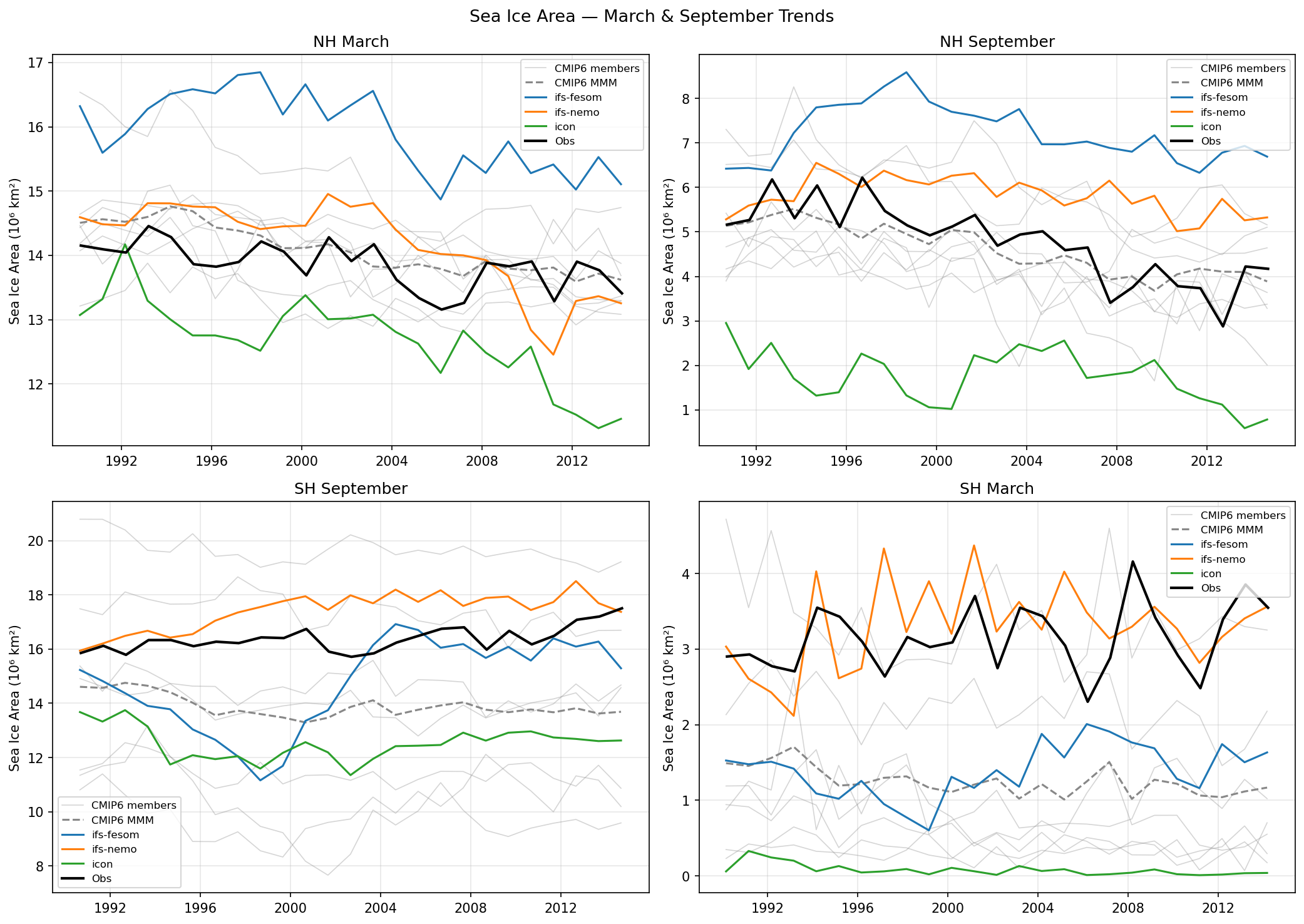
Sea Ice Area March & September Trends
| Variables | avg_siconc, avg_sithick |
|---|---|
| Models | MPI-ESM1-2-LR, ACCESS-ESM1-5, EC-Earth3, CNRM-CM6-1, CNRM-ESM2-1, INM-CM5-0, MRI-ESM2-0, ifs-fesom, ifs-nemo, icon |
| Reference Dataset | OSI_SAF |
| Units | 0-1 |
| Period | 1990–2014 |
Summary high
The figure evaluates the 1990–2014 interannual evolution of March and September sea ice area in both hemispheres, comparing three high-resolution DestinE models against OSI-SAF observations and a CMIP6 multi-model ensemble.
Key Findings
- IFS-NEMO exhibits the best overall performance, closely tracking observational magnitudes and interannual variability, particularly in the highly variable SH summer (March).
- ICON consistently and severely underestimates sea ice area across all seasons and both hemispheres, including a near-complete absence of SH summer sea ice.
- IFS-FESOM exhibits a distinct inter-hemispheric bias, significantly overestimating NH sea ice area in both seasons while underestimating SH summer sea ice.
Spatial Patterns
A clear declining trend is visible in the NH September (summer minimum) observations and most models, consistent with Arctic amplification. In contrast, the SH shows high interannual variability, particularly in March, with a slight upward trend in the September winter maximum during this specific historical period.
Model Agreement
The spread among the three high-resolution DestinE models is exceptionally large, often exceeding the spread of the traditional-resolution CMIP6 ensemble. IFS-NEMO shows high agreement with observations, while IFS-FESOM and ICON act as high and low outliers, respectively, in the Northern Hemisphere.
Physical Interpretation
The large model spread points to significant differences in coupled atmosphere-ocean-ice interactions. ICON's lack of SH summer sea ice suggests excessive atmospheric/oceanic heat fluxes into the ice or insufficient winter thickness buildup. IFS-FESOM's persistent positive bias in the NH may relate to insufficient oceanic heat transport into the Arctic or a surface cold bias. IFS-NEMO's strong performance suggests a better balance of dynamic ice transport and thermodynamic melt/growth.
Caveats
- The 25-year evaluation period (1990-2014) is relatively short for assessing long-term sea ice trends, particularly given strong decadal variability in the Southern Ocean.
- Sea ice area provides a two-dimensional view; evaluating sea ice thickness and volume is necessary to fully understand the underlying thermodynamic mass balance biases.
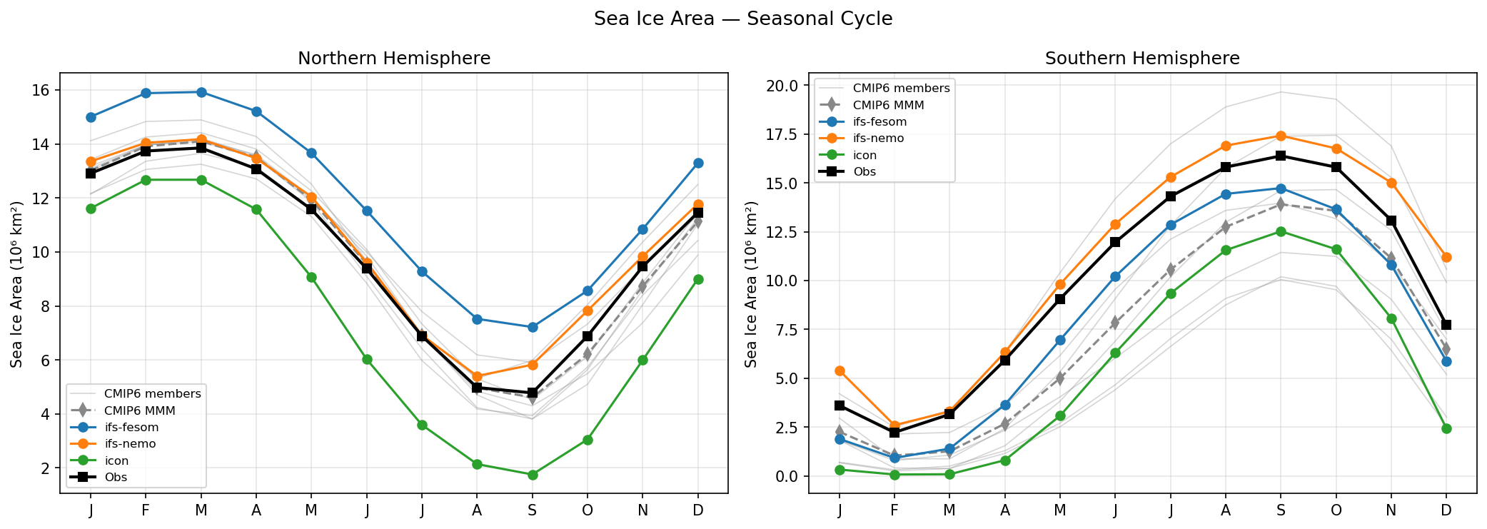
Sea Ice Area Seasonal Cycle
| Variables | avg_siconc, avg_sithick |
|---|---|
| Models | MPI-ESM1-2-LR, ACCESS-ESM1-5, EC-Earth3, CNRM-CM6-1, CNRM-ESM2-1, INM-CM5-0, MRI-ESM2-0, ifs-fesom, ifs-nemo, icon |
| Reference Dataset | OSI_SAF |
| Units | 0-1 |
| Period | 1990–2014 |
Summary high
Seasonal cycle of Northern and Southern Hemisphere sea ice area, comparing three high-resolution DestinE models against OSI-SAF observations and a subset of CMIP6 models over the 1990-2014 period.
Key Findings
- ifs-nemo exhibits excellent agreement with observations in the Northern Hemisphere and a slight positive bias during the growth phase and maximum in the Southern Hemisphere.
- icon shows a severe, systemic negative bias in sea ice area across both hemispheres year-round, with the Southern Hemisphere summer minimum approaching zero.
- ifs-fesom displays opposing hemispheric biases, overestimating sea ice area in the Northern Hemisphere while underestimating it in the Southern Hemisphere.
Spatial Patterns
All models correctly simulate the seasonal phase, with NH maxima in March and minima in September, and SH minima in February and maxima in September. However, the mean state offsets are substantial for ifs-fesom and icon throughout the entire annual cycle.
Model Agreement
Inter-model spread among the three DestinE models is notably large, particularly in the NH where it exceeds the spread of the plotted CMIP6 ensemble. ifs-nemo is the clear best performer. The CMIP6 MMM captures the NH well but exhibits a typical low bias in the SH maximum, which ifs-nemo improves upon, albeit by slightly overshooting.
Physical Interpretation
The massive divergence in sea ice area among models sharing the same atmosphere (IFS) but different ocean/ice components (NEMO vs FESOM) or a fully different coupled system (ICON) indicates that ocean/ice physics and tuning are the dominant drivers of these biases. ICON's global sea ice deficit suggests either excessive poleward oceanic heat transport or overly aggressive ice melt parameterizations. High horizontal resolution alone does not resolve these structural biases.
Caveats
- The analysis evaluates sea ice area only; assessing sea ice thickness and volume is necessary for a complete evaluation of the sea ice mass balance.
- The CMIP6 envelope shown represents only a subset of models, though the MMM provides a standard reference point.
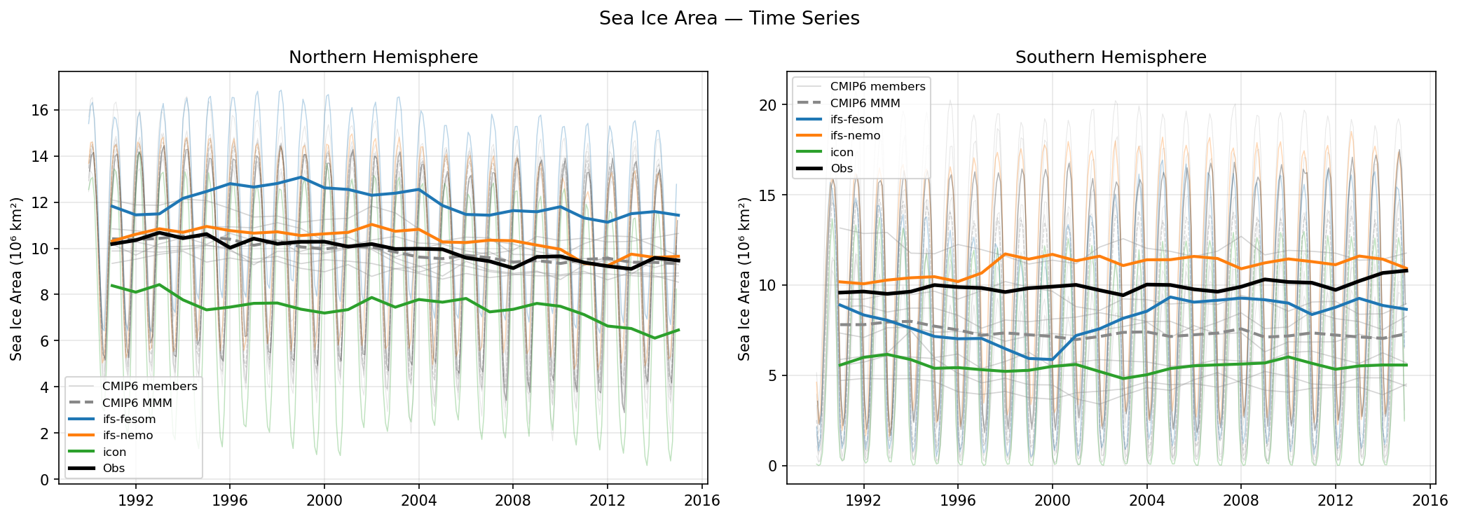
Sea Ice Area Time Series
| Variables | avg_siconc, avg_sithick |
|---|---|
| Models | MPI-ESM1-2-LR, ACCESS-ESM1-5, EC-Earth3, CNRM-CM6-1, CNRM-ESM2-1, INM-CM5-0, MRI-ESM2-0, ifs-fesom, ifs-nemo, icon |
| Reference Dataset | OSI_SAF |
| Units | 0-1 |
| Period | 1990–2014 |
Summary high
Time series of monthly and annual-mean sea ice area for the Northern and Southern Hemispheres spanning 1990-2015, comparing high-resolution DestinE models (IFS-FESOM, IFS-NEMO, ICON) against OSI-SAF observations and a CMIP6 multi-model ensemble.
Key Findings
- IFS-NEMO demonstrates excellent agreement with observations in the Northern Hemisphere but noticeably overestimates sea ice area in the Southern Hemisphere.
- ICON consistently and severely underestimates sea ice area in both hemispheres, with summer minimums frequently approaching zero.
- IFS-FESOM exhibits opposing hemispheric biases, overestimating sea ice area in the Northern Hemisphere while underestimating it in the Southern Hemisphere.
- The CMIP6 multi-model mean performs well in the NH but systematically underestimates SH sea ice area, a known bias in CMIP6.
Spatial Patterns
In the Northern Hemisphere, observations show a gradual decline in annual-mean sea ice area from roughly 10.5 to 9.5 million km² over the period, a trend broadly captured by the models. In the Southern Hemisphere, observed sea ice area remains relatively stable, but model mean states vary drastically, with annual means ranging from ~5 million km² (ICON) to ~12 million km² (IFS-NEMO). The seasonal cycle amplitudes (thin lines) also show massive divergence, particularly the excessively low summer minimums in ICON.
Model Agreement
There is poor inter-model agreement and a wide spread in both the mean state and the amplitude of the seasonal cycle. None of the high-resolution models consistently match observations across both hemispheres. IFS-NEMO performs best in the NH, but the CMIP6 MMM often outperforms the individual high-resolution models in capturing the baseline mean state.
Physical Interpretation
The large spread in sea ice area points to differing balances in surface radiation, ocean heat transport, and sea ice thermodynamics among the models. ICON's severe underestimation suggests a strong warm bias in polar regions, excessive ocean-to-ice heat flux, or a bias in ice albedo driving excessive summer melt. IFS-FESOM's hemispheric asymmetry may be tied to biases in the Atlantic Meridional Overturning Circulation (AMOC) or Antarctic Circumpolar Current (ACC) heat transports.
Caveats
- Differences between sea ice area and sea ice extent can influence comparisons if melt ponds or low-concentration regions are treated differently by models vs satellite retrievals.
- The CMIP6 MMM benefits from error cancellation, making it a challenging baseline for individual high-resolution models to beat in mean state metrics.
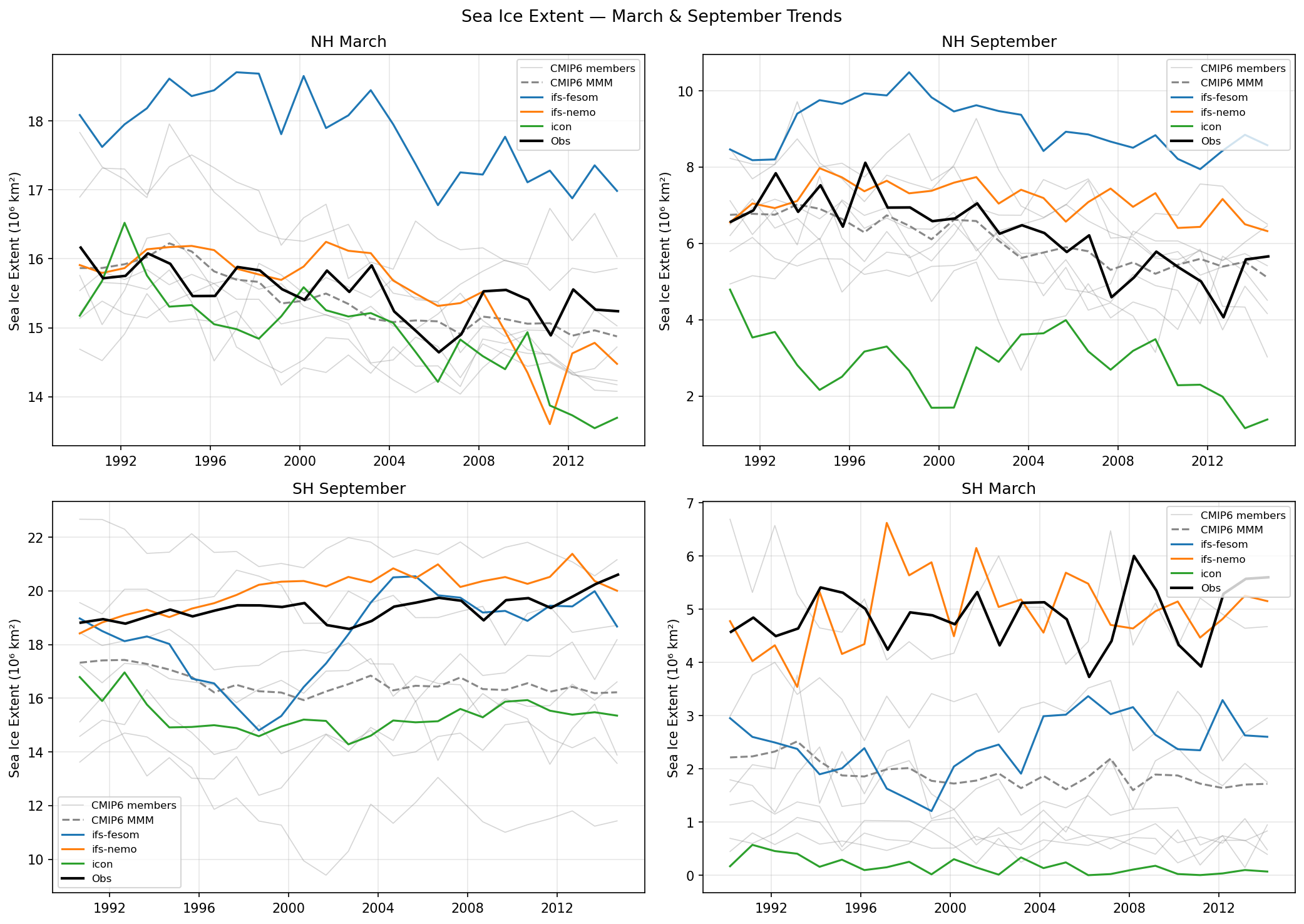
Sea Ice Extent March & September Trends
| Variables | avg_siconc, avg_sithick |
|---|---|
| Models | MPI-ESM1-2-LR, ACCESS-ESM1-5, EC-Earth3, CNRM-CM6-1, CNRM-ESM2-1, INM-CM5-0, MRI-ESM2-0, ifs-fesom, ifs-nemo, icon |
| Reference Dataset | OSI_SAF |
| Units | 0-1 |
| Period | 1990–2014 |
Summary high
The figure displays interannual variability and trends in March and September sea ice extent for the Northern and Southern Hemispheres from 1990 to 2014, comparing three high-resolution DestinE models against OSI-SAF observations and the CMIP6 ensemble.
Key Findings
- IFS-NEMO demonstrates the best overall performance, closely matching observed sea ice extent magnitudes and capturing interannual variability in both hemispheres and seasons.
- ICON severely underestimates summer sea ice extent in both hemispheres (NH September and SH March), approaching near ice-free conditions in the Antarctic summer.
- IFS-FESOM systematically overestimates Northern Hemisphere sea ice extent in both winter and summer, while exhibiting a strong, unrealistic decadal drift in Southern Hemisphere winter extent.
Spatial Patterns
In the Northern Hemisphere, observations show a declining trend, particularly in September, which all models capture with varying magnitudes. In the Southern Hemisphere September (winter maximum), observations indicate a slight increasing trend; IFS-NEMO reproduces this, whereas IFS-FESOM starts too low and drifts rapidly upward, and ICON remains systematically too low.
Model Agreement
Inter-model spread is remarkably large among the three high-resolution models, often exceeding the spread of the standard-resolution CMIP6 ensemble. IFS-NEMO agrees closely with observations and often outperforms the CMIP6 multi-model mean. Conversely, IFS-FESOM and ICON fall significantly outside the observational uncertainty and frequently outside the CMIP6 ensemble range, indicating substantial model biases.
Physical Interpretation
ICON's severe lack of summer sea ice points to excessive summer melting, likely driven by biases in the surface radiation budget (e.g., cloud radiative effects), ice albedo feedback, or excessive ocean-to-ice heat fluxes. IFS-FESOM's overestimation in the NH suggests insufficient oceanic heat transport into the Arctic or overly strong winter cooling. IFS-NEMO's strong performance suggests a better parameterized sea ice thermodynamic and dynamic coupling, leading to a more balanced surface energy budget.
Caveats
- The 25-year period (1990-2014) is relatively short for robustly distinguishing between decadal internal variability and long-term forced trends, particularly in the Southern Hemisphere.
- The models may not all be completely spun up, as evidenced by the large transient drift in IFS-FESOM's Southern Hemisphere September sea ice extent.
Sea Ice Extent Seasonal Cycle
| Variables | avg_siconc, avg_sithick |
|---|---|
| Models | MPI-ESM1-2-LR, ACCESS-ESM1-5, EC-Earth3, CNRM-CM6-1, CNRM-ESM2-1, INM-CM5-0, MRI-ESM2-0, ifs-fesom, ifs-nemo, icon |
| Reference Dataset | OSI_SAF |
| Units | 0-1 |
| Period | 1990–2014 |
Summary high
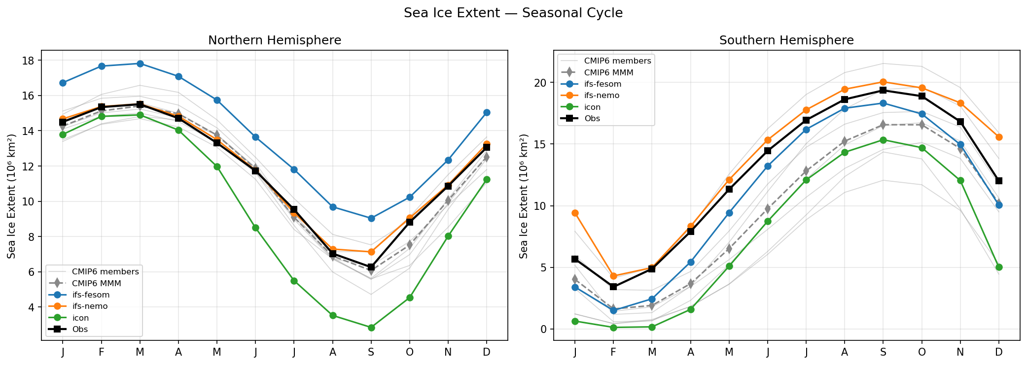
The figure displays the monthly climatological seasonal cycle of sea ice extent for the Northern and Southern Hemispheres, comparing three high-resolution DestinE models (ifs-fesom, ifs-nemo, icon) against OSI-SAF observations and a CMIP6 ensemble over the 1990-2014 period.
Key Findings
- ifs-nemo exhibits the highest fidelity to observations in both hemispheres, closely tracking the observed seasonal amplitude and phase.
- ifs-fesom demonstrates a persistent positive sea ice extent bias year-round in the Northern Hemisphere (+2 to +3 million km²) and a negative bias in the Southern Hemisphere.
- icon systematically underestimates sea ice extent year-round in both hemispheres, with severe underestimation during the summer minima (down to ~2.8 million km² in the NH and near zero in the SH).
Spatial Patterns
In the Northern Hemisphere (March maximum, September minimum), the DestinE models bracket the observations with systematic offsets, preserving the seasonal cycle shape but shifting the mean state. In the Southern Hemisphere (February minimum, September maximum), observations peak at ~19.5 million km². ifs-nemo slightly overestimates this peak, while ifs-fesom, icon, and particularly the CMIP6 multi-model mean significantly underestimate the winter/spring extent.
Model Agreement
Inter-model agreement among the high-resolution DestinE models is poor, as they diverge significantly in their mean states. ifs-nemo shows excellent agreement with observations. The CMIP6 multi-model mean captures the NH seasonal cycle reasonably well but struggles significantly in the SH, where it heavily underestimates winter sea ice extent—a common deficiency in standard-resolution CMIP models.
Physical Interpretation
The persistent, year-round biases seen in ifs-fesom and icon suggest underlying mean-state errors rather than purely seasonal process deficiencies. These are likely driven by biases in ocean poleward heat transport (e.g., Atlantic Meridional Overturning Circulation strength affecting the NH, or Antarctic Circumpolar Current dynamics affecting the SH), or atmospheric forcing (such as downwelling longwave radiation and cloud radiative effects). The exaggerated summer minimum in icon suggests a strong ice-albedo feedback exacerbating the initial negative bias.
Caveats
- Sea ice extent is purely a two-dimensional area metric; a model matching extent perfectly (like ifs-nemo) may still harbor significant biases in sea ice thickness or volume.
- The 1990-2014 period includes rapid transient climate change, particularly the sharp decline in Arctic sea ice, which is averaged out in this stationary climatological view.
Sea Ice Extent Time Series
| Variables | avg_siconc, avg_sithick |
|---|---|
| Models | MPI-ESM1-2-LR, ACCESS-ESM1-5, EC-Earth3, CNRM-CM6-1, CNRM-ESM2-1, INM-CM5-0, MRI-ESM2-0, ifs-fesom, ifs-nemo, icon |
| Reference Dataset | OSI_SAF |
| Units | 0-1 |
| Period | 1990–2014 |
Summary high
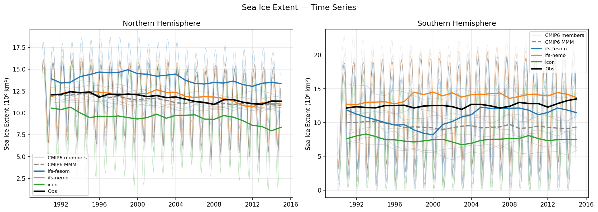
Time series of monthly and annual-mean sea ice extent for the Northern and Southern Hemispheres, comparing DestinE high-resolution models against OSI-SAF observations and a CMIP6 multi-model ensemble.
Key Findings
- ifs-nemo demonstrates excellent agreement with observed annual-mean sea ice extent in the Northern Hemisphere, though it slightly overestimates extent in the Southern Hemisphere.
- icon systematically underestimates sea ice extent in both hemispheres, with Southern Hemisphere summer extent reaching near-zero values.
- ifs-fesom significantly overestimates Northern Hemisphere sea ice extent and exhibits anomalous decadal-scale variability (a pronounced dip and recovery) in the Southern Hemisphere.
- The high-resolution DestinE models exhibit a much larger inter-model spread in mean state sea ice extent than the CMIP6 multi-model mean.
Spatial Patterns
In the Northern Hemisphere, observations show a gradual decline in sea ice extent over the 1990-2015 period. icon captures a declining trend but starts from a biased-low state, while ifs-nemo tracks both the mean state and the observed decline well. In the Southern Hemisphere, observations remain relatively stable, but models show large mean state offsets, with icon and the CMIP6 MMM severely underestimating the total extent.
Model Agreement
Inter-model agreement is low among the DestinE models, with annual means spanning roughly 8 to 15 million km² in the NH and 7 to 14 million km² in the SH. ifs-nemo performs best overall against observations, while icon and ifs-fesom bracket the observations with substantial negative and positive biases, respectively.
Physical Interpretation
The severe underestimation of sea ice in icon, particularly the nearly ice-free SH summers, suggests excessive oceanic heat transport to the poles, a strong positive ice-albedo feedback, or an overly warm atmospheric state. Conversely, ifs-fesom's NH overestimation likely stems from regional cold biases or insufficient oceanic heat convergence. The erratic SH behavior in ifs-fesom may indicate issues with deep convection or Southern Ocean stratification adjustments in the model.
Caveats
- The relatively short 25-year period makes it difficult to separate secular forced trends from internal decadal variability, particularly for the anomalous SH behavior in ifs-fesom.
- Comparisons with the CMIP6 MMM should note that the MMM inherently smooths out individual model variability, leading to artificially lower interannual variance compared to single realizations.
Sea Ice Volume March & September Trends
| Variables | avg_siconc, avg_sithick |
|---|---|
| Models | MPI-ESM1-2-LR, ACCESS-ESM1-5, EC-Earth3, CNRM-CM6-1, CNRM-ESM2-1, INM-CM5-0, MRI-ESM2-0, ifs-fesom, ifs-nemo, icon |
| Reference Dataset | PSC |
| Units | 0-1 |
| Period | 1990–2014 |
Summary high
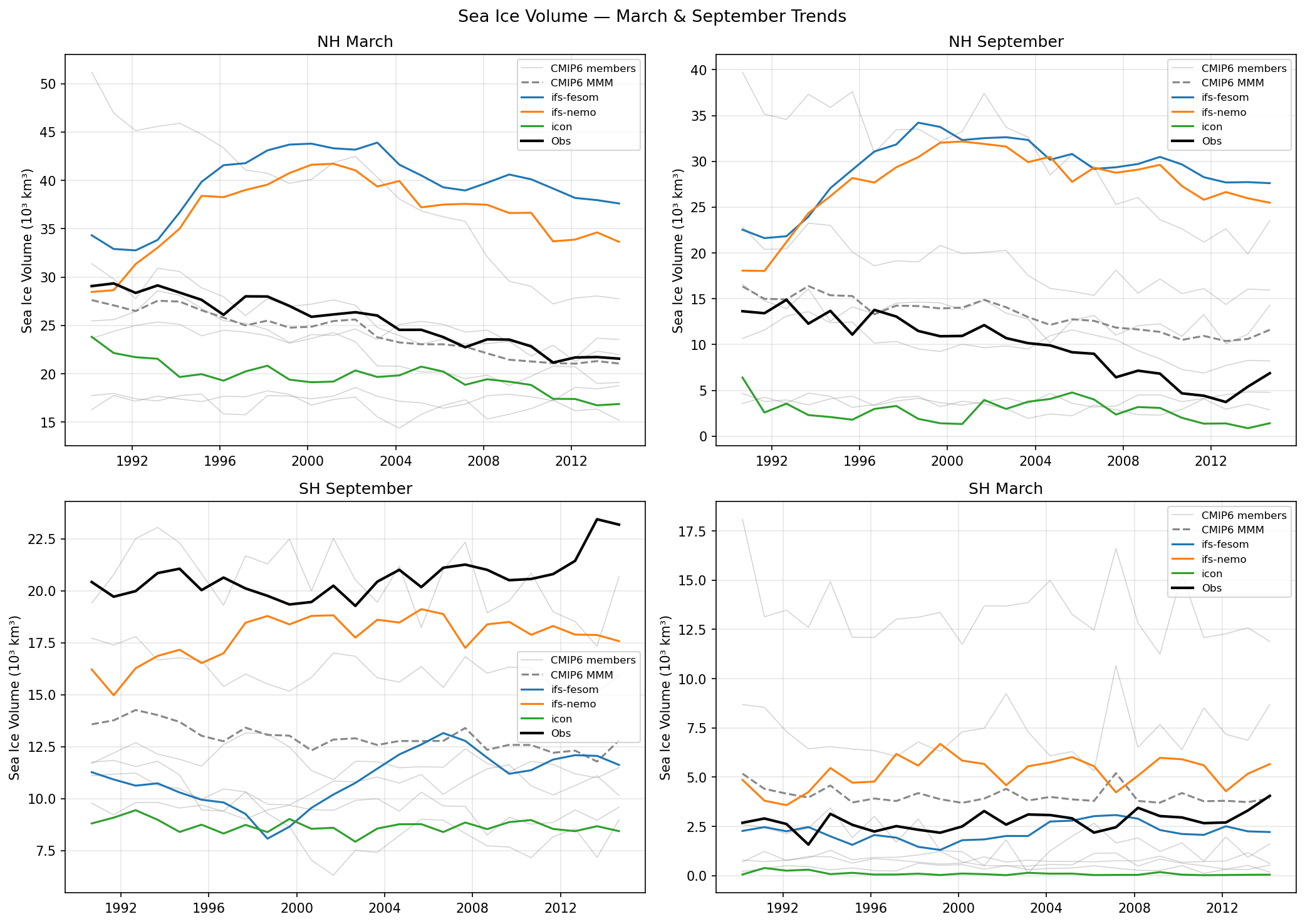
The figure presents the 1990-2014 evolution of Arctic (NH) and Antarctic (SH) sea ice volume during their respective annual maximum and minimum months, comparing high-resolution DestinE models against observations and a CMIP6 ensemble.
Key Findings
- IFS-FESOM and IFS-NEMO severely overestimate NH sea ice volume in both March and September, exhibiting an unrealistic volume increase during the 1990s and failing to capture the observed steep decline.
- ICON consistently underestimates sea ice volume across all hemispheres and seasons, approaching near-zero volume during the SH March minimum.
- All three high-resolution models significantly underestimate SH September (winter maximum) sea ice volume compared to observations, with ICON showing the largest deficit.
- The CMIP6 multi-model mean closely tracks observations in the NH, outperforming all three un-tuned high-resolution DestinE models.
Spatial Patterns
In the Northern Hemisphere, IFS-FESOM and IFS-NEMO show massive positive volume biases (exceeding +10-15 x 10³ km³ in September), while ICON shows a persistent negative bias. In the Southern Hemisphere, all models exhibit negative volume biases during the winter maximum (September), but diverge during the summer minimum (March) where IFS-NEMO overestimates and ICON underestimates volume.
Model Agreement
There is poor agreement between the high-resolution models and observations, as well as poor inter-model agreement. The IFS-driven models group together with strong positive NH biases, while ICON stands alone with systemic negative biases. The mature CMIP6 ensemble shows much better agreement with observations, highlighting the challenges in tuning new high-resolution systems.
Physical Interpretation
The severe overestimation of NH volume by IFS models suggests excessive winter thermodynamic ice growth, insufficient summer melt, or anomalous ice piling, likely driven by atmospheric cold biases or cloud-radiation errors. Conversely, ICON's global ice deficit implies a systemic positive surface energy balance anomaly over polar oceans or overly vigorous ocean mixing that enhances basal melt. The IFS models' failure to reproduce the strong downward trend in NH September volume indicates a flawed sensitivity to recent warming or a prolonged spin-up adjustment.
Caveats
- Observational sea ice volume is not directly measured but derived from reanalysis systems (e.g., PIOMAS/GIOMAS) that assimilate concentration and model thickness, meaning 'Obs' carries substantial uncertainty.
- CMIP6 models benefit from extensive historical tuning, whereas the DestinE models are newer, coupled at much higher resolutions, and may not yet have fully calibrated polar parameterizations or reached equilibrium.
Sea Ice Volume Seasonal Cycle
| Variables | avg_siconc, avg_sithick |
|---|---|
| Models | MPI-ESM1-2-LR, ACCESS-ESM1-5, EC-Earth3, CNRM-CM6-1, CNRM-ESM2-1, INM-CM5-0, MRI-ESM2-0, ifs-fesom, ifs-nemo, icon |
| Reference Dataset | PSC |
| Units | 0-1 |
| Period | 1990–2014 |
Summary high
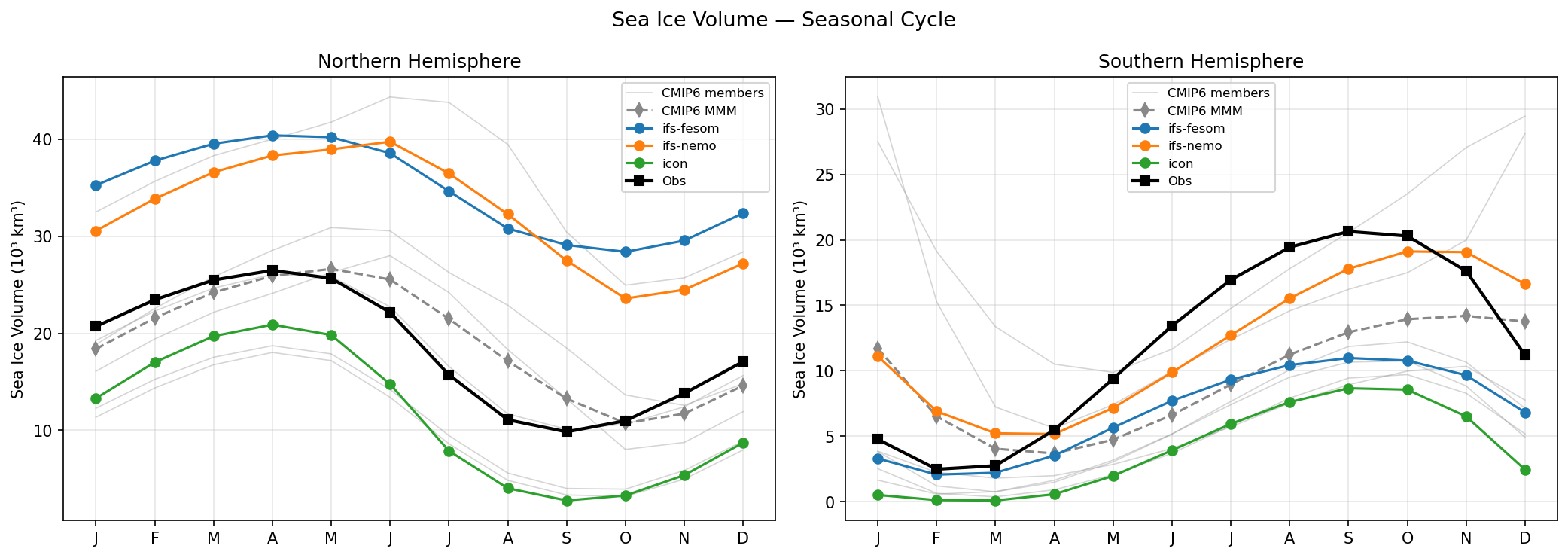
Seasonal cycle of Northern and Southern Hemisphere sea ice volume for high-resolution models (IFS-FESOM, IFS-NEMO, ICON) compared to CMIP6 models and observations (PIOMAS/GIOMAS).
Key Findings
- IFS-FESOM and IFS-NEMO severely overestimate Northern Hemisphere sea ice volume throughout the year (positive bias of ~10-15 x10³ km³).
- ICON underestimates Northern Hemisphere sea ice volume, particularly in the summer/autumn minimum, but tracks closer to the CMIP6 multi-model mean.
- In the Southern Hemisphere, all high-resolution models underestimate sea ice volume compared to observations, with ICON showing the strongest negative bias.
- The CMIP6 multi-model mean captures the observed Northern Hemisphere seasonal cycle reasonably well but underestimates Southern Hemisphere volume.
Spatial Patterns
Northern Hemisphere volume peaks in April-May and reaches a minimum in September-October. Southern Hemisphere volume peaks in September-October and reaches a minimum in February-March. The amplitude of the seasonal cycle is captured well across models, but absolute values are biased.
Model Agreement
Poor agreement between high-resolution models and observations. IFS-FESOM and IFS-NEMO cluster together with a massive positive bias in the NH, while ICON sits much lower. In the SH, IFS-NEMO performs best among the high-resolution models, but still underestimates the peak volume. CMIP6 spread is very large, but the MMM performs better than the individual high-res models in the NH.
Physical Interpretation
The large positive bias in IFS-FESOM/NEMO NH sea ice volume suggests either excessive ice growth (due to negative surface energy budget biases, e.g., insufficient downward longwave radiation or too much sea ice albedo) or insufficient melting/export. The SH underestimation across all models (CMIP6 and high-res) suggests a common deficiency in simulating Antarctic sea ice, possibly related to Southern Ocean stratification, ocean heat transport, or wind forcing.
Caveats
- Observations for sea ice volume are derived from reanalyses (PIOMAS/GIOMAS) rather than direct satellite measurements, so they carry considerable uncertainty themselves.
- The 'Obs' label likely refers to PIOMAS/GIOMAS despite the metadata listing PSC (which is for concentration).
Sea Ice Volume Time Series
| Variables | avg_siconc, avg_sithick |
|---|---|
| Models | MPI-ESM1-2-LR, ACCESS-ESM1-5, EC-Earth3, CNRM-CM6-1, CNRM-ESM2-1, INM-CM5-0, MRI-ESM2-0, ifs-fesom, ifs-nemo, icon |
| Reference Dataset | PSC |
| Units | 0-1 |
| Period | 1990–2014 |
Summary high
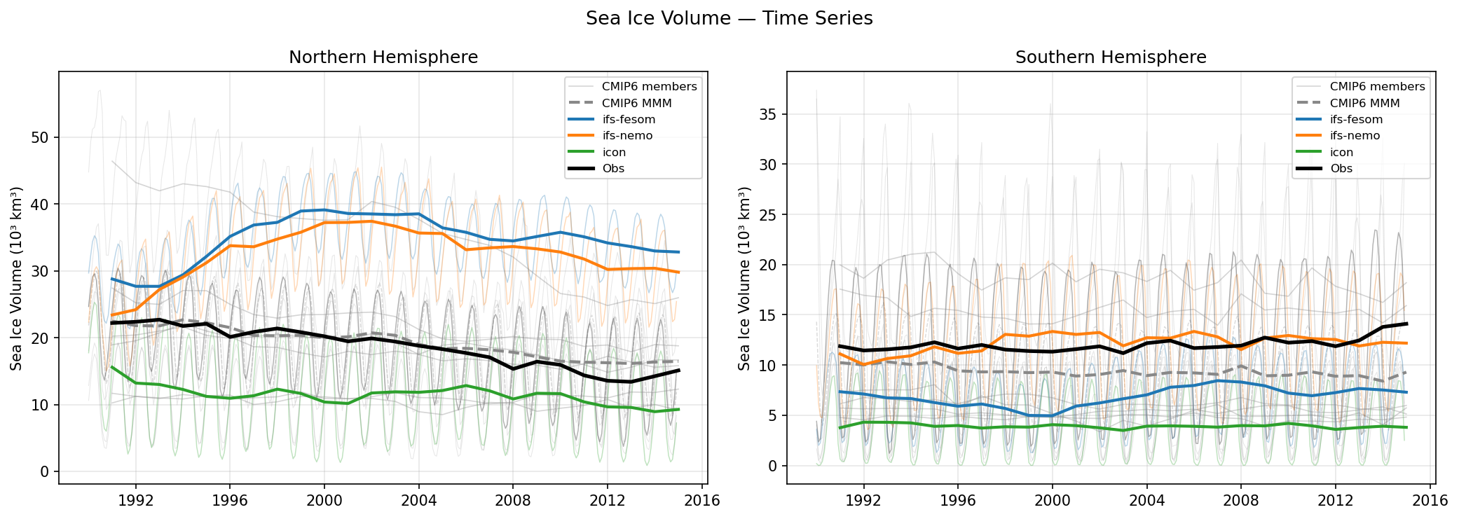
Time series of Northern and Southern Hemisphere sea ice volume from 1990 to 2015, comparing high-resolution DestinE models (IFS-FESOM, IFS-NEMO, ICON) against observational estimates and the CMIP6 multi-model mean.
Key Findings
- IFS-FESOM and IFS-NEMO significantly overestimate Northern Hemisphere sea ice volume by up to a factor of two, while ICON consistently underestimates it.
- In the Southern Hemisphere, IFS-NEMO closely matches the observational mean, whereas IFS-FESOM and ICON severely underestimate sea ice volume.
- The high-resolution models exhibit large inter-model spread and generally do not outperform the standard-resolution CMIP6 multi-model mean, which tracks observations more closely, particularly in the NH.
- IFS-FESOM and IFS-NEMO show an unphysical increase in NH sea ice volume during the 1990s before declining, failing to capture the observed steady downward trend.
Spatial Patterns
In the Northern Hemisphere, observations exhibit a clear, steady declining trend in sea ice volume over the 1990-2014 period. IFS-FESOM and IFS-NEMO fail to capture this initial trajectory, showing anomalous growth until roughly 2000 before starting to decline. In the Southern Hemisphere, observations show a relatively stable mean state with a slight increase towards the end of the period. While IFS-NEMO captures the SH mean magnitude, IFS-FESOM and ICON show flat, negatively biased trajectories.
Model Agreement
Inter-model agreement among the high-resolution DestinE models is very poor, indicating large structural or parametric uncertainties in representing polar sea ice. IFS-FESOM and IFS-NEMO share similar positive biases in the NH but diverge significantly in the SH. ICON is a consistent outlier, simulating the lowest sea ice volume globally. Overall, model-observation agreement is poor, with only IFS-NEMO in the SH showing good alignment with the observational mean state.
Physical Interpretation
The large deviations in sea ice volume point to underlying biases in sea ice thickness, likely driven by errors in oceanic heat transport, surface radiative fluxes (e.g., due to cloud biases), or sea ice dynamics. ICON's global underestimation suggests excessive heat transport to the poles or excessive surface melting. The pronounced initial growth of NH sea ice in IFS-FESOM and IFS-NEMO strongly suggests a model spin-up issue or a severe adjustment to the coupled forcing, rather than a physical response to historical climate forcing.
Caveats
- Observational estimates for sea ice volume (typically derived from assimilative models like PIOMAS in the NH and GIOMAS in the SH) carry significant uncertainties due to the lack of continuous, basin-wide sea ice thickness observations.
- The 'Obs' dataset is not explicitly named in the figure legend for volume, requiring assumption that standard reanalysis products are used.
Arctic Sea Ice Concentration
| Variables | avg_siconc |
|---|---|
| Models | ifs-fesom, ifs-nemo, icon |
| Reference Dataset | OSI_SAF |
| Units | 0-1 |
| Period | 1990–2014 |
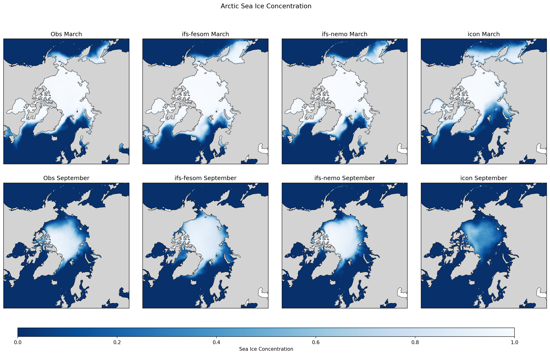
Summary high
Polar stereographic maps comparing Arctic sea ice concentration in March (maximum) and September (minimum) across three high-resolution models and OSI-SAF observations.
Key Findings
- IFS-FESOM and IFS-NEMO generally overestimate sea ice extent in both March and September, particularly in the marginal seas.
- ICON systematically underestimates sea ice concentration and extent across both seasons, exhibiting a severe low-concentration bias in the central Arctic during September.
- During the March maximum, ICON fails to capture sea ice in the Sea of Okhotsk and Bering Sea, whereas IFS-FESOM and IFS-NEMO extend ice too far south in the Labrador, Greenland, and Barents Seas.
- During the September minimum, IFS-FESOM and IFS-NEMO simulate an overly solid and extensive ice pack, while ICON simulates a highly diffuse ice pack that is significantly thinner/less concentrated than observed.
Spatial Patterns
In March, observational ice cover fills the Arctic basin and marginal seas. IFS-FESOM and IFS-NEMO show positive extent biases in the Atlantic sector (Greenland/Barents Seas) and Labrador Sea. ICON shows negative biases in the Pacific sector (Bering/Okhotsk Seas). In September, observations show the ice pack retreated to the central Arctic. IFS-FESOM and IFS-NEMO maintain too much ice along the Siberian and Alaskan coasts. ICON's September ice pack is uniformly too low in concentration (~0.4-0.6) across the entire central Arctic basin.
Model Agreement
Models diverge significantly from observations and each other. IFS-FESOM and IFS-NEMO share similar positive biases in extent and concentration, likely linked to their shared IFS atmospheric component. ICON completely diverges, showing severe negative concentration and extent biases in both seasons.
Physical Interpretation
The positive sea ice biases in IFS-FESOM and IFS-NEMO suggest either insufficient oceanic heat transport into the Arctic (e.g., weak Atlantic water inflow) or overly cold atmospheric surface conditions. Conversely, ICON's severe underestimation of September ice concentration and lack of winter marginal sea ice points to excessive ocean-to-ice heat fluxes, excessive downward surface shortwave radiation during summer, or an overly strong ice-albedo feedback driving excessive summer melt.
Caveats
- Passive microwave satellite observations (OSI-SAF) can underestimate summer sea ice concentration due to surface melt ponds being misidentified as open water, though this cannot fully explain the extreme negative bias seen in ICON.
- The analysis period (1990-2014) encompasses a period of rapid observed Arctic sea ice decline, so climatological averages may smooth over significant temporal trends that differ between models.
Antarctic Sea Ice Concentration
| Variables | avg_siconc |
|---|---|
| Models | ifs-fesom, ifs-nemo, icon |
| Reference Dataset | OSI_SAF |
| Units | 0-1 |
| Period | 1990–2014 |
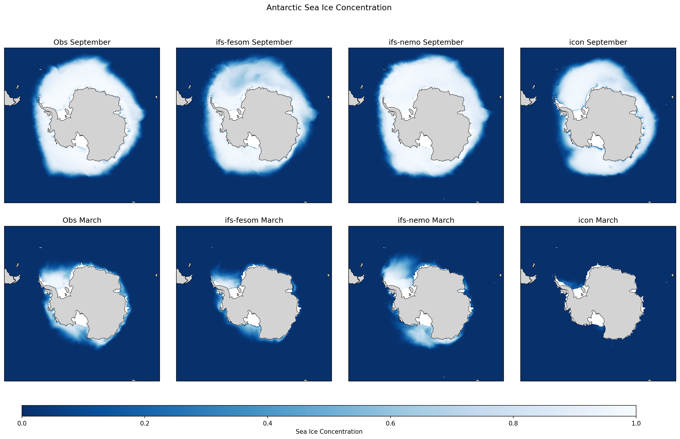
Summary high
Polar stereographic maps of Antarctic sea ice concentration for September (annual maximum) and March (annual minimum), comparing IFS-FESOM, IFS-NEMO, and ICON against OSI-SAF observations.
Key Findings
- ICON severely underestimates Antarctic sea ice extent and concentration in both the winter maximum (September) and summer minimum (March).
- IFS-FESOM and IFS-NEMO capture the broad spatial pattern of the September maximum extent, exhibiting good agreement with observations.
- During the March minimum, IFS-NEMO overestimates sea ice in the Ross and Amundsen Seas, whereas IFS-FESOM underestimates the residual ice pack compared to observations.
Spatial Patterns
In September, observations show a vast sea ice pack extending outward from the continent, which is well simulated by the IFS models, though IFS-FESOM shows slightly higher concentrations at the margins. ICON's September ice edge is drastically retreated toward the coast across all sectors. In March, observed sea ice is mostly confined to the Weddell Sea and parts of the Amundsen/Bellingshausen Seas. IFS-NEMO retains excessive ice in the Ross Sea, IFS-FESOM is largely restricted to a reduced Weddell Sea pack, and ICON is virtually ice-free.
Model Agreement
There is strong divergence between ICON and the two IFS models. While IFS-FESOM and IFS-NEMO generally agree on the winter sea ice state, they exhibit notable regional differences in the location and amount of surviving summer ice (e.g., in the Ross Sea).
Physical Interpretation
The severe lack of sea ice in ICON points to a pronounced warm bias in the Southern Ocean, likely driven by excessive vertical ocean mixing, insufficient upper-ocean stratification, or excessive downward longwave radiation. The regional biases in the IFS models during summer (e.g., IFS-NEMO's excess in the Ross Sea) may relate to the representation of local ocean circulation patterns, such as the Ross Gyre, or differences in the sea ice albedo feedback during the melt season.
Caveats
- Satellite retrievals of sea ice concentration can have higher uncertainties during the summer melt season.
- The 1990-2014 period is relatively short and may be influenced by strong internal decadal variability in the Southern Ocean.
Arctic Sea Ice Thickness (m)
| Variables | avg_sithick |
|---|---|
| Models | ifs-fesom, ifs-nemo, icon |
| Reference Dataset | PSC |
| Units | m |
| Period | 1990–2014 |
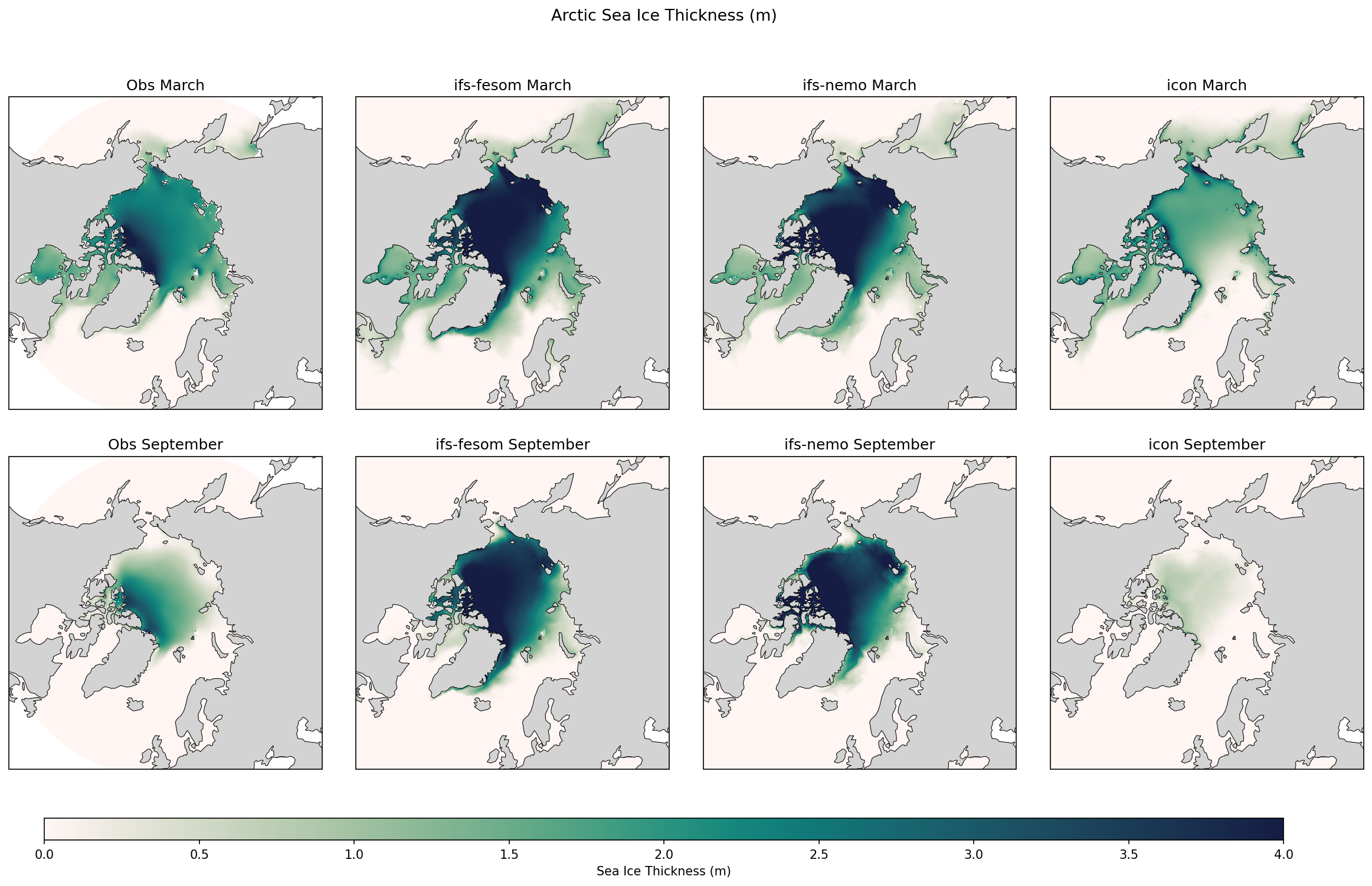
Summary high
Spatial maps of Arctic sea ice thickness in March and September highlight severe overestimations in IFS-FESOM and IFS-NEMO compared to observations, while ICON shows a highly realistic distribution.
Key Findings
- IFS-FESOM and IFS-NEMO massively overestimate sea ice thickness across the central Arctic Basin in both March and September, with vast regions exceeding 4 meters.
- ICON accurately captures the observed spatial gradients in March thickness, particularly the thickest ice north of Greenland and the Canadian Archipelago.
- During the September minimum, the IFS-coupled models retain an unrealistic amount of extremely thick ice, whereas ICON closely matches the observed remnant ice distribution.
Spatial Patterns
Observations display a distinct transpolar thickness gradient, with ice >3m packed against northern Greenland and the Canadian Archipelago, thinning towards the Eurasian marginal seas. IFS-FESOM and IFS-NEMO completely obscure this gradient with widespread >4m ice covering the entire central basin. ICON successfully reproduces the observed gradient in March and appropriately localizes the thickest surviving ice in September.
Model Agreement
There is strong divergence between the models. IFS-FESOM and IFS-NEMO agree in their severe positive thickness biases. ICON is the outlier among the models but exhibits the highest agreement with observations.
Physical Interpretation
The excessive ice in IFS-FESOM and IFS-NEMO points to fundamental imbalances in surface energy fluxes (e.g., inadequate summer shortwave absorption or excessive winter longwave cooling) or deficient sea ice dynamics (e.g., insufficient export through Fram Strait or excessive dynamic ridging). ICON's performance suggests a better tuned surface radiation balance and more realistic ice rheology and transport.
Caveats
- Observational sea ice thickness datasets prior to the CryoSat-2 era (post-2010) often rely on models or reanalyses (like PIOMAS), carrying significant uncertainties.
- Satellite-derived thickness observations in summer months have high uncertainty due to the presence of surface melt ponds confounding radar and laser altimetry retrievals.
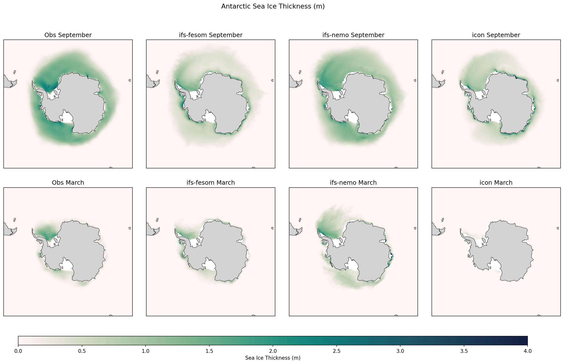
Antarctic Sea Ice Thickness (m)
| Variables | avg_sithick |
|---|---|
| Models | ifs-fesom, ifs-nemo, icon |
| Reference Dataset | PSC |
| Units | m |
| Period | 1990–2014 |
Summary high
Spatial maps of Antarctic sea ice thickness for September (maximum) and March (minimum) comparing three high-resolution models against observations.
Key Findings
- ICON severely underestimates both sea ice extent and thickness, resulting in an almost completely ice-free Antarctic in March.
- IFS-NEMO captures the most realistic spatial distribution and thickness of ice, particularly retaining thick ice in the Weddell Sea.
- IFS-FESOM simulates less and thinner ice than IFS-NEMO, presenting a generalized negative thickness bias, but performs significantly better than ICON.
Spatial Patterns
In September (maximum), observations show thick ice (> 2 m) concentrated in the Weddell and Amundsen/Bellingshausen Seas with broad overall extent. IFS-NEMO replicates this broad extent and regional thickness reasonably well. IFS-FESOM shows a narrower extent and thinner ice overall. ICON's September ice is anomalously thin and tightly confined to the coast. In March (minimum), observations retain substantial thick ice in the western Weddell Sea; IFS-NEMO maintains some of this pack ice, IFS-FESOM retains very little, and ICON is virtually ice-free.
Model Agreement
Inter-model agreement is poor for Antarctic sea ice thickness. IFS-NEMO agrees best with the observational spatial pattern and magnitude. ICON exhibits a drastic negative bias in both seasons. IFS-FESOM falls between the two but leans toward a negative bias.
Physical Interpretation
The profound differences between IFS-FESOM and IFS-NEMO, which share the same atmospheric model (IFS), indicate that the choice of ocean and sea ice component strongly governs the Southern Ocean sea ice state. ICON's severe lack of ice suggests a strong warm bias in Southern Ocean sea surface temperatures, potentially driven by excessive vertical mixing of deep Circumpolar Deep Water (CDW) or biases in cloud-radiative forcing.
Caveats
- Antarctic sea ice thickness observations are notoriously poorly constrained and often rely on reanalysis systems (e.g., GIOMAS), which is evident from the non-physical 'ringing' artifacts in the observational panels.
- Internal variability in the Southern Ocean is high, and the 1990-2014 period may be subject to decadal trends that models out of phase with observations might not capture.