Evaluation Seasonal Cycle CMIP6
CMIP6 Multi-Model Mean Context
Comparison with CMIP6 ensemble mean from 10 members.
Contributing models: ACCESS-ESM1-5, AWI-CM-1-1-MR, CNRM-CM6-1, CNRM-ESM2-1, EC-Earth3, GISS-E2-1-G, INM-CM5-0, IPSL-CM6A-LR, MPI-ESM1-2-LR, MRI-ESM2-0
Synthesis
Related diagnostics
10m U Wind Seasonal Cycle
| Variables | avg_10u |
|---|---|
| Models | ifs-fesom, ifs-nemo, icon, MPI-ESM1-2-LR, GISS-E2-1-G, IPSL-CM6A-LR, ACCESS-ESM1-5, EC-Earth3, CNRM-CM6-1, AWI-CM-1-1-MR, CNRM-ESM2-1, INM-CM5-0, MRI-ESM2-0 |
| Reference Dataset | ERA5 |
| Units | m/s |
| Period | 1990–2014 |
Summary high
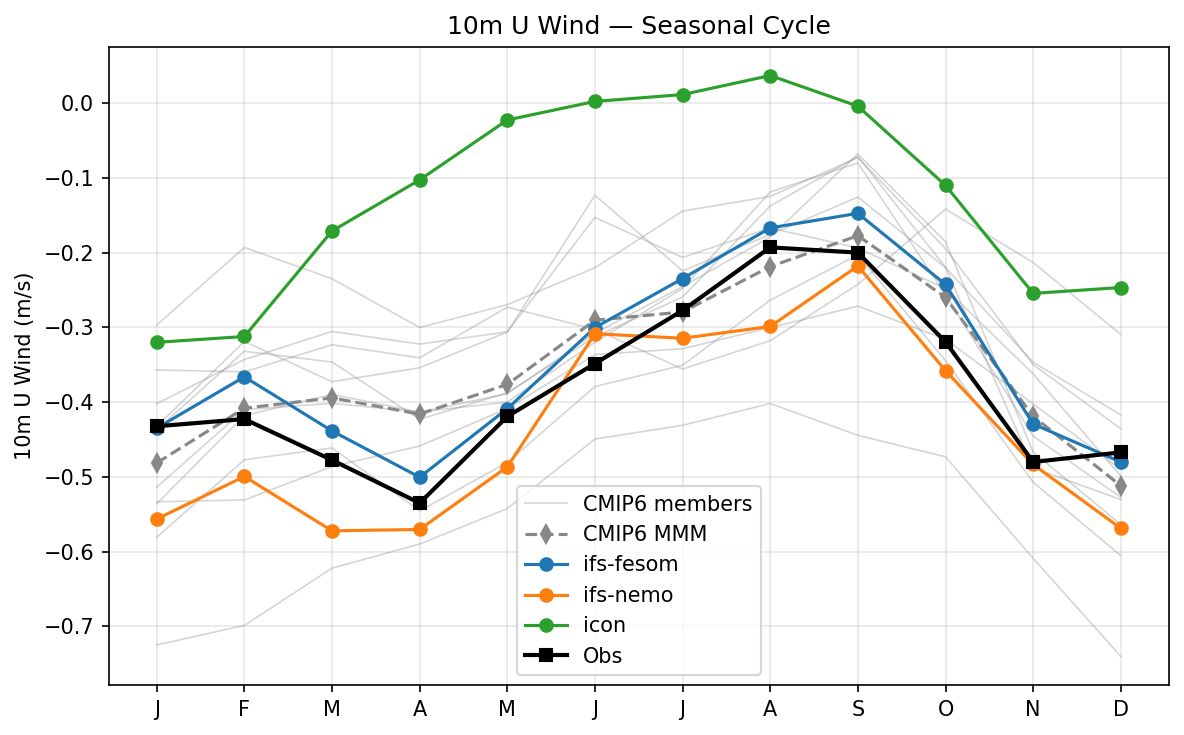
The figure illustrates the seasonal cycle of global mean 10m zonal wind (U wind) for three DestinE high-resolution models compared to ERA5 reanalysis and the CMIP6 ensemble.
Key Findings
- ICON exhibits a persistent positive bias (too westerly) of ~0.15 to 0.25 m/s throughout the year.
- IFS-FESOM tracks ERA5 observations very closely, particularly from June through November.
- IFS-NEMO accurately captures the seasonal phase but maintains a consistent negative offset (too easterly) of roughly -0.05 to -0.1 m/s.
- The CMIP6 multi-model mean generally matches ERA5 but slightly underestimates the strength of the global easterly flow in boreal spring.
Spatial Patterns
The temporal pattern features a globally averaged negative (easterly) 10m U wind, reflecting a net easterly momentum at the surface. The cycle has a minimum in April (strongest net easterlies, ~-0.55 m/s) and a maximum in September (weakest net easterlies, ~-0.2 m/s).
Model Agreement
IFS-FESOM shows excellent agreement with ERA5. IFS-NEMO and ICON bracket the observations with systematic negative and positive biases, respectively. Inter-model spread among the DestinE models is notably large, with ICON diverging significantly from the CMIP6 envelope.
Physical Interpretation
Global mean 10m U wind represents the delicate net balance between tropical trade winds (easterlies) and mid-latitude westerlies. ICON's positive bias suggests its mid-latitude westerlies are overly strong or its tropical trades are too weak. Because IFS-NEMO and IFS-FESOM share the same atmospheric component (IFS), their divergence implies that differences in the coupled ocean models (NEMO vs FESOM) and resulting sea surface temperature or current feedback patterns significantly modulate global low-level atmospheric circulation.
Caveats
- Averaging globally conceals large regional compensating biases; a model could have severe errors in both westerlies and easterlies that cancel out in the global mean.
- ERA5 10m winds are a reanalysis product reliant on the assimilating model's boundary layer physics, introducing uncertainty especially over data-sparse open ocean regions like the Southern Ocean.
10m V Wind Seasonal Cycle
| Variables | avg_10v |
|---|---|
| Models | ifs-fesom, ifs-nemo, icon, MPI-ESM1-2-LR, GISS-E2-1-G, IPSL-CM6A-LR, ACCESS-ESM1-5, EC-Earth3, CNRM-CM6-1, AWI-CM-1-1-MR, CNRM-ESM2-1, INM-CM5-0, MRI-ESM2-0 |
| Reference Dataset | ERA5 |
| Units | m/s |
| Period | 1990–2014 |
Summary high
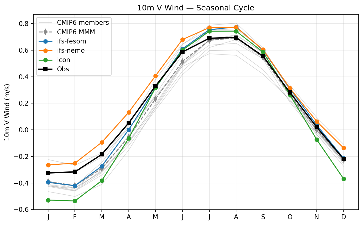
The figure illustrates the seasonal cycle of the global mean 10m meridional (V) wind, capturing the transition from net northerly flow in boreal winter to net southerly flow in boreal summer, driven by the seasonal migration of cross-equatorial circulations.
Key Findings
- All models successfully capture the phase of the seasonal cycle, which peaks negatively in January/February and positively in July/August.
- The high-resolution DestinE models (ifs-fesom, ifs-nemo, icon) generally overestimate the positive (southerly) peak in boreal summer compared to ERA5.
- The 'icon' model exhibits an amplified seasonal cycle, producing overly strong northerly winds in boreal winter and overly strong southerly winds in boreal summer.
- The 'ifs-nemo' model displays a systematic positive (southerly) bias throughout almost the entire year relative to observations.
Spatial Patterns
As a global mean diagnostic, spatial information is aggregated; however, the temporal pattern shows a robust transition from approximately -0.3 m/s in January to +0.7 m/s in July, reflecting hemispheric asymmetry and the dominance of specific seasonal low-level wind regimes.
Model Agreement
Phase agreement is excellent across all models and ERA5. However, amplitude agreement varies significantly: the CMIP6 multi-model mean tracks the observations relatively well but slightly overestimates the winter minimum. The DestinE models show greater divergence, with 'icon' overestimating the cycle amplitude and 'ifs-nemo' showing a persistent positive offset. 'ifs-fesom' aligns closely with the CMIP6 MMM during boreal winter but aligns more with the other DestinE models in overestimating the summer peak.
Physical Interpretation
The non-zero global mean 10m V wind and its strong seasonal cycle are primarily governed by the seasonal migration of the Intertropical Convergence Zone (ITCZ) and the associated cross-equatorial lower-tropospheric flow (e.g., the Somali Jet during the Asian summer monsoon). An amplified seasonal cycle (as seen in 'icon') or systematic offsets (as seen in 'ifs-nemo') suggest biases in the intensity of the Hadley circulation branches, the representation of monsoonal flow strength, or the annual mean latitudinal position of the ITCZ.
Caveats
- A global mean metric can obscure large compensating regional biases in meridional wind (e.g., between the Pacific and Atlantic basins).
- Area-averaging of near-zero global quantities makes the metric sensitive to small, systematic boundary layer parameterization differences between models.
2m Temperature Seasonal Cycle
| Variables | avg_2t |
|---|---|
| Models | ifs-fesom, ifs-nemo, icon, MPI-ESM1-2-LR, GISS-E2-1-G, IPSL-CM6A-LR, ACCESS-ESM1-5, EC-Earth3, CNRM-CM6-1, AWI-CM-1-1-MR, CNRM-ESM2-1, FGOALS-g3, INM-CM5-0, MRI-ESM2-0 |
| Reference Dataset | ERA5 |
| Units | K |
| Period | 1990–2014 |
Summary high
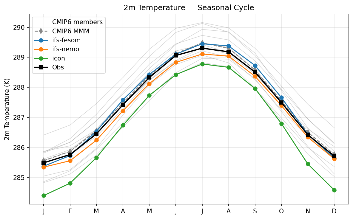
The figure displays the global mean 2m temperature seasonal cycle, demonstrating that while all high-resolution models accurately capture the seasonal phase and amplitude, ICON and IFS-NEMO exhibit systematic year-round cold biases compared to ERA5 observations.
Key Findings
- IFS-FESOM shows excellent agreement with ERA5 and the CMIP6 multi-model mean, with only marginal deviations.
- IFS-NEMO displays a consistent, slight cold bias of approximately 0.2-0.3 K throughout the entire seasonal cycle.
- ICON exhibits a pronounced and persistent cold bias of roughly 1.0 K, placing it near the lower bound of the traditional-resolution CMIP6 ensemble spread.
Spatial Patterns
The diagnostic evaluates the global mean temporal (seasonal) pattern, characterized by a peak in July (~289.3 K) and a minimum in January (~285.5 K), driven by the larger landmass in the Northern Hemisphere responding more strongly to seasonal variations in insolation.
Model Agreement
All high-resolution models and CMIP6 members strongly agree on the phase and amplitude (~3.8 K peak-to-trough) of the seasonal cycle. However, there is significant inter-model spread in the absolute global mean temperature, with ICON diverging the most from observations while IFS-FESOM closely tracks the ERA5 benchmark.
Physical Interpretation
The persistent, year-round cold biases in ICON and IFS-NEMO point to systematic offsets in the global top-of-atmosphere or surface energy budgets. This is frequently driven by excessive shortwave reflection from clouds (cloud-radiative effects), overly reflective surface albedos (particularly in sea-ice or snow-covered regions), or biases in turbulent heat fluxes at the ocean-atmosphere interface. Because the seasonal amplitude is correct, the transient response to solar forcing is well-simulated, but the baseline equilibrium state is too cold.
Caveats
- Global mean time series can obscure large regional compensating errors (e.g., a warm bias in the tropics cancelling out a cold bias in the mid-latitudes).
- Comparisons of absolute global mean temperature are highly sensitive to the spatial masking and interpolation methods used when translating model native grids to the observation grid.
Surface Sensible Heat Flux Seasonal Cycle
| Variables | avg_ishf |
|---|---|
| Models | ifs-fesom, ifs-nemo, icon |
| Reference Dataset | ERA5 |
| Units | W/m2 |
| Period | 1990–2014 |
Summary high
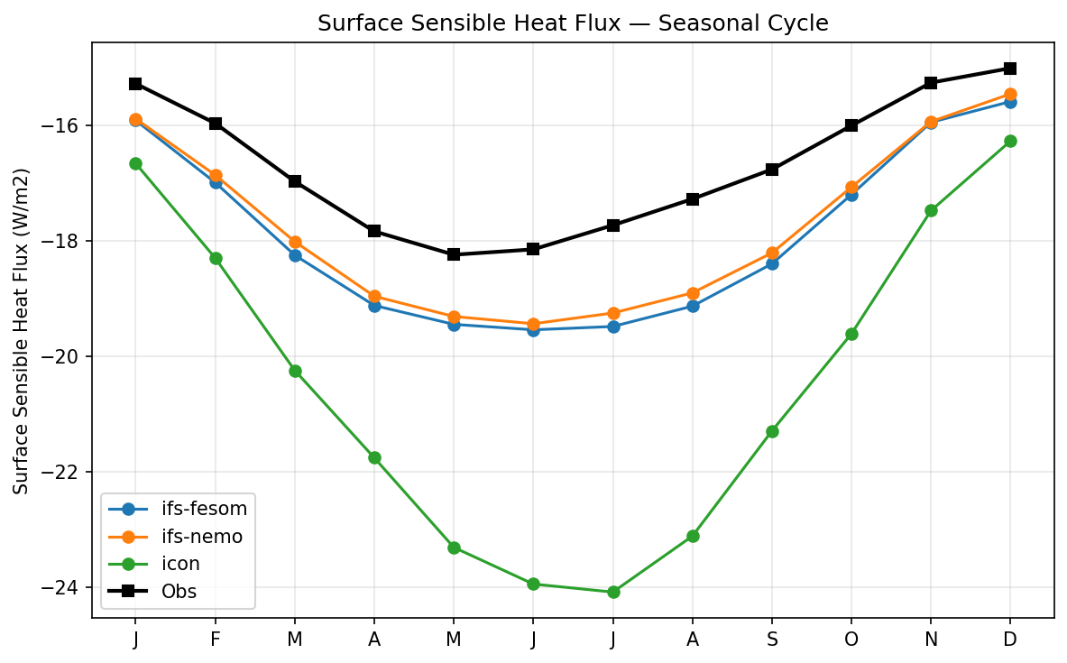
Global mean seasonal cycle of surface sensible heat flux, showing all models overestimate the magnitude of upward flux compared to ERA5, with ICON exhibiting the strongest seasonal bias.
Key Findings
- All models correctly simulate the seasonal phase, with peak upward sensible heat flux (most negative values) occurring during boreal summer (May-July).
- IFS-FESOM and IFS-NEMO show a consistent, moderate overestimation of upward flux magnitude (~1-2 W/m2) year-round.
- The ICON model exhibits a much larger bias, overestimating the upward flux magnitude by up to 6 W/m2 during the boreal summer maximum.
Spatial Patterns
The temporal pattern exhibits a distinct peak in magnitude (most negative values) during the Northern Hemisphere summer months (May-August), reflecting the dominance of NH landmass surface heating in the global sensible heat flux budget. Minimum magnitude occurs in December and January.
Model Agreement
IFS-FESOM and IFS-NEMO agree very closely with each other, tracking the observational seasonal cycle well but with a persistent negative offset. ICON diverges significantly from both the IFS-based models and observations, exhibiting an exaggerated seasonal amplitude.
Physical Interpretation
The global seasonal cycle is largely driven by Northern Hemisphere land surfaces, which experience strong insolation and surface heating during boreal summer, driving strong upward sensible heat fluxes (denoted by negative values). ICON's pronounced overestimation during summer suggests potential issues with land-atmosphere coupling, boundary layer parameterizations, or overly dry soils that partition available energy heavily towards sensible rather than latent heat. The nearly identical behavior of the two IFS models demonstrates that this global diagnostic is governed by their shared atmospheric component rather than the ocean model.
Caveats
- ERA5 is used as the observational reference; as a reanalysis product, its surface fluxes rely heavily on model parameterizations and are subject to uncertainties.
- Global mean time series obscure spatial heterogeneity, potentially masking compensating regional biases between land and ocean domains.
Mean Sea Level Pressure Seasonal Cycle
| Variables | avg_msl |
|---|---|
| Models | ifs-fesom, ifs-nemo, icon, MPI-ESM1-2-LR, GISS-E2-1-G, IPSL-CM6A-LR, ACCESS-ESM1-5, EC-Earth3, CNRM-CM6-1, AWI-CM-1-1-MR, CNRM-ESM2-1, FGOALS-g3, INM-CM5-0, MRI-ESM2-0 |
| Reference Dataset | ERA5 |
| Units | Pa |
| Period | 1990–2014 |
Summary high
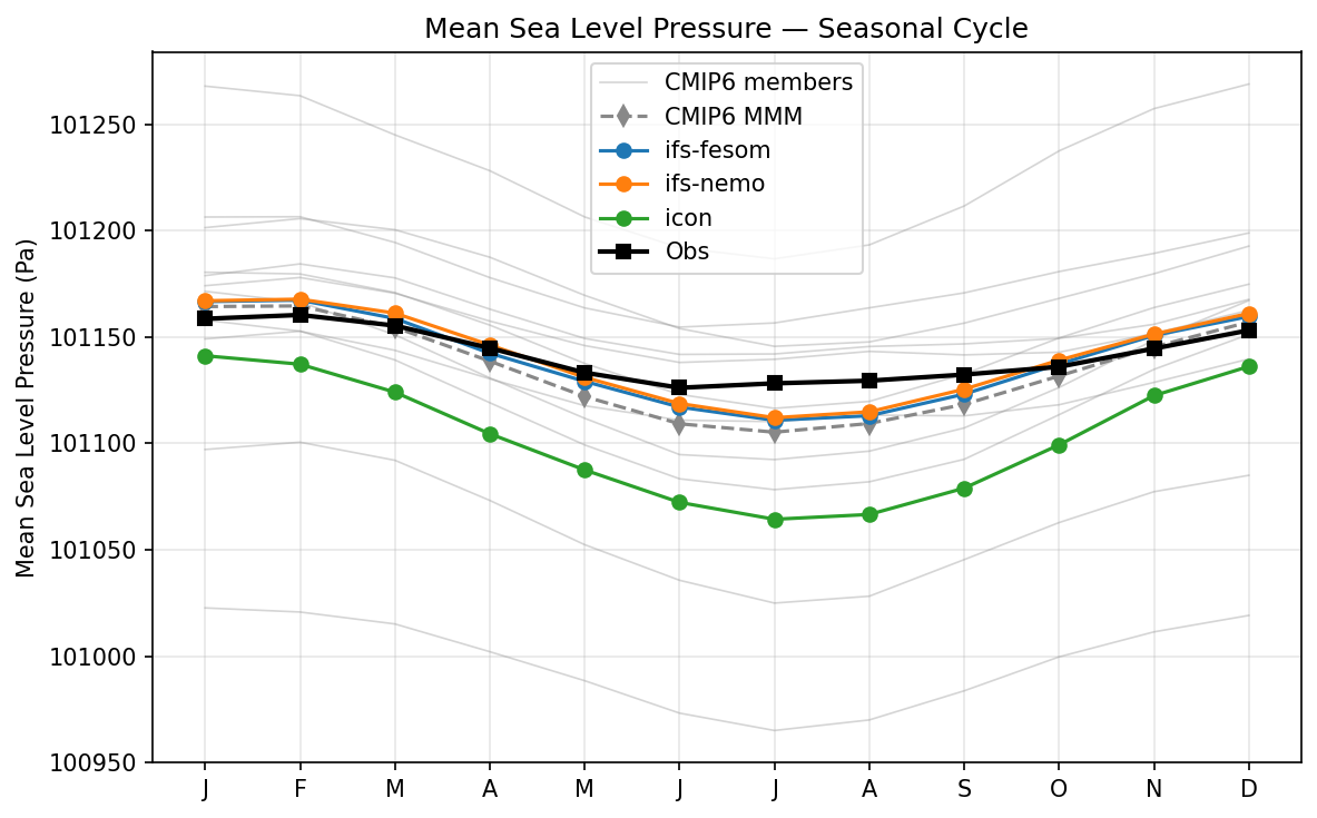
The figure displays the global mean seasonal cycle of Mean Sea Level Pressure (MSLP), illustrating that high-resolution IFS models closely replicate observations, while ICON shows a systematic offset and standard-resolution CMIP6 models exhibit massive inter-model spread.
Key Findings
- IFS-FESOM and IFS-NEMO closely track the observed ERA5 MSLP, capturing the mean magnitude well but slightly overestimating the seasonal amplitude with a minor negative bias (~20 Pa) in boreal summer.
- ICON systematically underestimates global mean MSLP by 20 to 70 Pa throughout the year, although it correctly reproduces the seasonal phase and amplitude.
- Individual CMIP6 models display an extraordinarily large spread in global mean MSLP (spanning over 300 Pa), highlighting significant baseline inconsistencies across traditional-resolution models.
Spatial Patterns
Temporal patterns show a global mean MSLP maximum in boreal winter (January-February, ~101160 Pa) and a minimum in boreal summer (July-August, ~101130 Pa). This seasonal phase is consistently captured across all high-resolution models, the CMIP6 multi-model mean, and observations.
Model Agreement
IFS-FESOM and IFS-NEMO exhibit excellent agreement with each other and with ERA5. ICON agrees in seasonal phase but diverges significantly in absolute magnitude. The CMIP6 multi-model mean tracks observations closely, but this masks the huge underlying spread among individual CMIP6 members, indicating poor inter-model agreement in baseline atmospheric mass.
Physical Interpretation
Although global dry atmospheric mass is largely conserved, global mean MSLP exhibits a seasonal cycle due to the temperature-dependent extrapolation of surface pressure down to sea level over topography. During boreal winter, the Northern Hemisphere's large landmasses cool rapidly; the resulting cold, dense 'artificial' air mass below ground raises the global mean MSLP. The large baseline spread across CMIP6 models is primarily driven by differences in the initialization of global dry air mass and variations in topographic extrapolation schemes, whereas the IFS models appear more accurately calibrated to reanalysis mass totals.
Caveats
- Global mean MSLP is an extrapolated quantity highly sensitive to the temperature reduction algorithms used over mountainous terrain; differences between models and ERA5 may reflect algorithmic choices rather than true physical biases.
- Offsets in global mean pressure of this magnitude (tens of Pascals) are negligible compared to regional dynamical pressure gradients and do not necessarily degrade the model's simulated atmospheric circulation.
Surface Downwelling Longwave Seasonal Cycle
| Variables | avg_sdlwrf |
|---|---|
| Models | ifs-fesom, ifs-nemo, icon, MPI-ESM1-2-LR, GISS-E2-1-G, IPSL-CM6A-LR, ACCESS-ESM1-5, EC-Earth3, CNRM-CM6-1, AWI-CM-1-1-MR, CNRM-ESM2-1, FGOALS-g3, INM-CM5-0, MRI-ESM2-0 |
| Reference Dataset | ERA5 |
| Units | W/m2 |
| Period | 1990–2014 |
Summary high
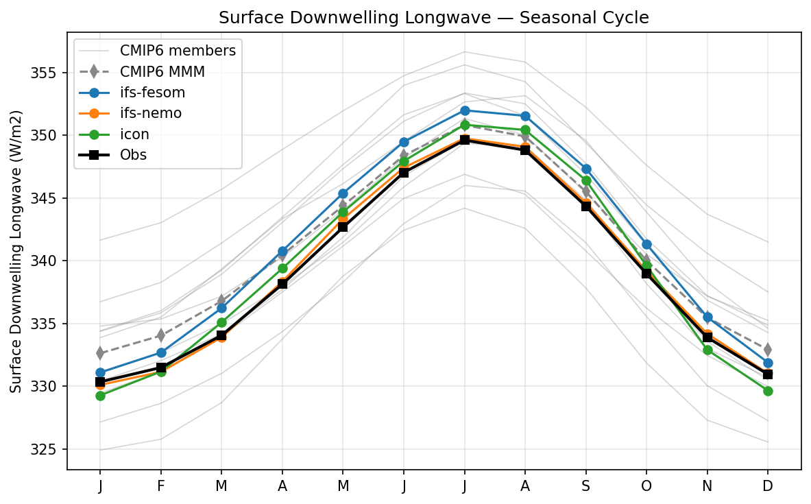
The figure illustrates the global mean seasonal cycle of surface downwelling longwave radiation, comparing three high-resolution DestinE models against ERA5 reanalysis and the CMIP6 ensemble spread.
Key Findings
- ifs-nemo exhibits exceptional agreement with ERA5 observations throughout the entire seasonal cycle.
- The three high-resolution models show a significantly reduced spread and generally better observational agreement compared to the wide distribution of individual CMIP6 models.
- ifs-fesom demonstrates a systematic positive bias of approximately 1-2 W/m2 year-round, while icon closely tracks observations with only minor seasonal deviations.
Spatial Patterns
The temporal pattern shows a global maximum in July-August (~350 W/m2) and a minimum in December-January (~330 W/m2). This cycle is dominated by the Northern Hemisphere, where the larger landmass drives higher summer atmospheric temperatures and increased water vapor, consequently peaking the global downwelling longwave emission.
Model Agreement
Inter-model agreement among the high-resolution models is strong, tightly clustering near the observations compared to the broad CMIP6 spread. Model-observation agreement is highest for ifs-nemo, followed closely by icon. ifs-fesom and the CMIP6 multi-model mean both exhibit consistent positive biases relative to ERA5.
Physical Interpretation
Surface downwelling longwave radiation is highly sensitive to lower tropospheric temperature, column water vapor, and low-level cloud fraction and optical depth. The near-perfect tracking by ifs-nemo implies a highly accurate simulated climatology of boundary layer thermodynamics and cloud properties. The persistent positive bias in ifs-fesom suggests a globally warmer or moister lower troposphere, or an overestimation of low cloud cover.
Caveats
- Global mean time series can mask compensating regional biases; a model with perfect global mean agreement may still have significant spatial errors.
- ERA5 is a reanalysis product, and while highly constrained, its surface radiative fluxes contain model-dependent uncertainties and should ideally be cross-referenced with direct observational products like CERES.
Surface Downwelling Shortwave Seasonal Cycle
| Variables | avg_sdswrf |
|---|---|
| Models | ifs-fesom, ifs-nemo, icon, MPI-ESM1-2-LR, GISS-E2-1-G, IPSL-CM6A-LR, ACCESS-ESM1-5, EC-Earth3, CNRM-CM6-1, AWI-CM-1-1-MR, CNRM-ESM2-1, FGOALS-g3, INM-CM5-0, MRI-ESM2-0 |
| Reference Dataset | ERA5 |
| Units | W/m2 |
| Period | 1990–2014 |
Summary high
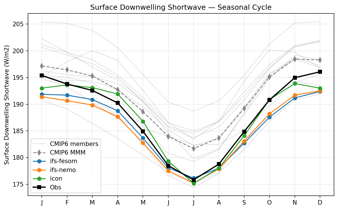
The figure illustrates the global mean seasonal cycle of surface downwelling shortwave radiation, comparing three high-resolution DestinE models against ERA5 observations and the CMIP6 ensemble.
Key Findings
- High-resolution DestinE models (IFS-FESOM, IFS-NEMO, ICON) exhibit a persistent negative bias of 2-5 W/m2 during the boreal winter and spring months compared to ERA5.
- The CMIP6 multi-model mean shows a systematic positive bias year-round, indicating that the DestinE models have reversed the common 'too bright' surface bias prevalent in coarser-resolution models.
- All three DestinE models converge and show excellent agreement with observations during the boreal summer months (June to August).
Spatial Patterns
The temporal pattern shows a global mean shortwave maximum in December/January and a minimum in July, driven by Earth's orbital eccentricity and hemispheric asymmetries in land/ocean and cloud cover. DestinE models accurately capture the phase of this cycle but with a slight downward shift in the annual mean.
Model Agreement
Inter-model spread among the three DestinE models is exceptionally tight (~2 W/m2) compared to the vast spread seen in the CMIP6 ensemble (~20 W/m2). ICON is slightly closer to observations from January to April, but all three models exhibit a similar trajectory, particularly their strong convergence with observations in July.
Physical Interpretation
The widespread reduction in surface downwelling shortwave in DestinE models relative to the CMIP6 MMM suggests changes in cloud radiative effects. Higher resolution models likely resolve convective clouds and marine stratocumulus more effectively, increasing cloud optical thickness or fraction. While this corrects the CMIP6 positive bias, the resulting slight negative bias implies that these models may produce clouds that are slightly too reflective or widespread, particularly in the Southern Hemisphere which dominates the global mean during austral summer.
Caveats
- Global mean time series can mask significant regional compensating errors (e.g., negative tropical biases canceling positive mid-latitude biases).
- ERA5 surface shortwave radiation is a modeled product within the reanalysis and may itself contain biases compared to direct satellite observations like CERES.
Surface Latent Heat Flux Seasonal Cycle
| Variables | avg_slhtf |
|---|---|
| Models | ifs-fesom, ifs-nemo, icon |
| Reference Dataset | ERA5 |
| Units | W/m2 |
| Period | 1990–2014 |
Summary high
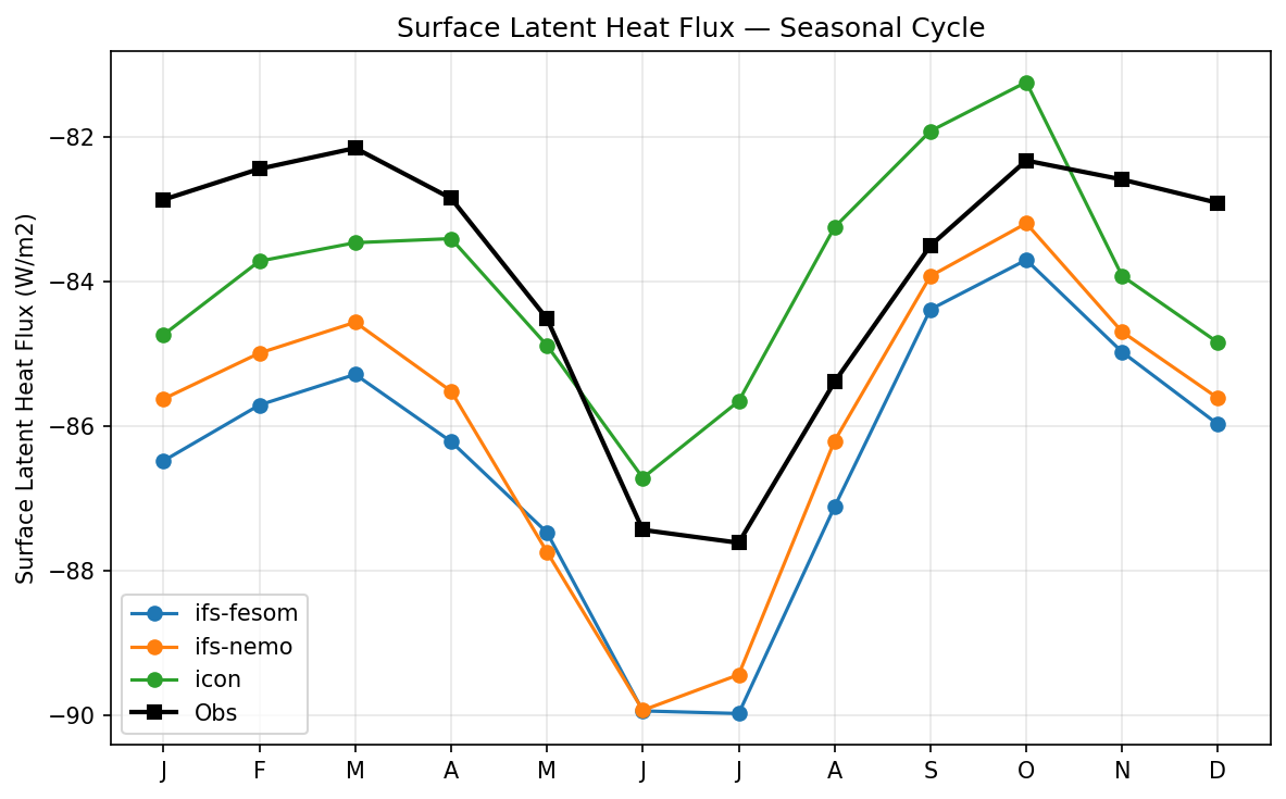
The figure illustrates the global mean seasonal cycle of surface latent heat flux, comparing the IFS-FESOM, IFS-NEMO, and ICON high-resolution models against ERA5 reanalysis data. While all models capture the semi-annual temporal structure, they exhibit distinct biases in the overall magnitude of the upward moisture fluxes.
Key Findings
- Both IFS-driven models (FESOM and NEMO) consistently overestimate the magnitude of the upward latent heat flux (exhibiting more negative values) throughout the entire year compared to ERA5.
- The ICON model best captures the observational magnitude during the boreal summer minimum (June-July) but underestimates the upward flux magnitude (less negative values) during the boreal autumn (September-November).
- All models successfully reproduce the phase and timing of the global seasonal cycle, including the weakest upward fluxes in March and October, and the strongest upward flux in June-July.
Spatial Patterns
The temporal pattern is characterized by a bimodal or semi-annual cycle in the global mean. The strongest global surface latent heat flux (most negative, ~ -87.5 W/m2 in observations) occurs during June and July, largely driven by Northern Hemisphere summer evaporation, while the weakest fluxes occur in the transition seasons of March and October.
Model Agreement
The IFS-FESOM and IFS-NEMO models show high inter-model agreement, sharing a nearly identical seasonal trajectory and a persistent 1-3 W/m2 overestimation of the flux magnitude. ICON diverges significantly from the IFS models, showing better agreement with ERA5 in JJA but poorer agreement in SON. No single model consistently matches the ERA5 baseline across all seasons.
Physical Interpretation
In standard meteorological convention, negative surface latent heat flux denotes upward energy transfer (evaporation). The systematically more negative values in the IFS models indicate excessive global evaporation. This is likely driven by overly strong parameterized near-surface wind speeds, warm sea surface temperature biases, or differences in the bulk aerodynamic transfer coefficients. ICON's underestimation of the flux magnitude in boreal autumn could stem from differences in the representation of Northern Hemisphere land-surface drying or shifts in tropical convection and wind patterns.
Caveats
- Global mean time series can obscure significant regional compensating errors (e.g., opposing biases over land versus ocean).
- ERA5 is a reanalysis product relying on parameterized model physics for surface fluxes, meaning it is not a direct observation and carries its own inherent uncertainties.
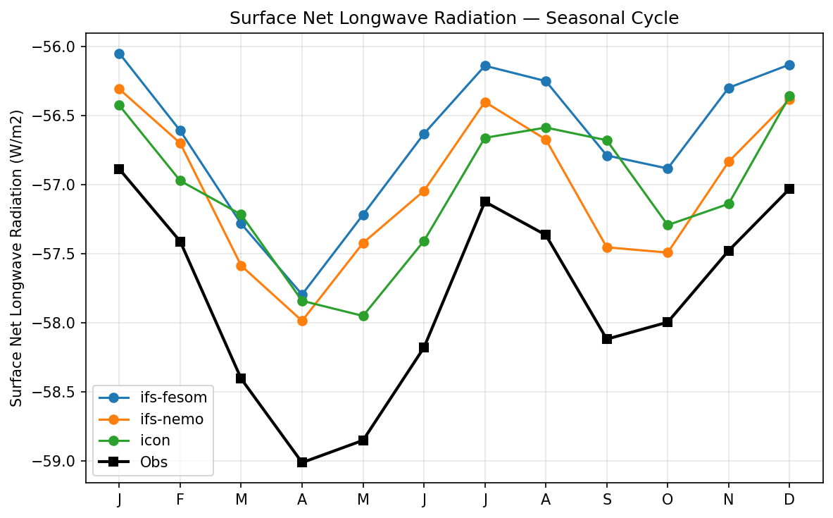
Surface Net Longwave Radiation Seasonal Cycle
| Variables | avg_snlwrf |
|---|---|
| Models | ifs-fesom, ifs-nemo, icon |
| Reference Dataset | ERA5 |
| Units | W/m2 |
| Period | 1990–2014 |
Summary high
The figure displays the seasonal cycle of global mean surface net longwave radiation, showing that all three high-resolution models systematically overestimate the net longwave flux (i.e., less negative values, indicating reduced surface heat loss) compared to ERA5 reanalysis.
Key Findings
- All models exhibit a persistent positive bias of ~0.5 to 1.5 W/m2 throughout the year compared to ERA5, implying an underestimation of net surface longwave cooling.
- While models broadly capture the primary seasonal minimum (strongest surface cooling) in April, they fail to adequately reproduce the observed secondary minimum in September-October.
- The two IFS-based models (ifs-fesom and ifs-nemo) produce a pronounced peak (weakest cooling) in July that is much less prominent in both the observations and the ICON model.
Spatial Patterns
The observed temporal cycle features dual minima (strongest net upward flux) in April and September/October, and maxima in January and July. The models accurately capture the spring minimum but misrepresent the late summer/autumn progression, with IFS models strongly overestimating the July maximum and ICON showing a flatter June-August trajectory.
Model Agreement
All models agree on the systematic positive bias (insufficient surface cooling) relative to ERA5. Inter-model agreement in seasonal phasing is high between the two IFS-coupled models (ifs-fesom and ifs-nemo), whereas ICON diverges during the boreal summer months.
Physical Interpretation
The persistent positive bias (less net upward longwave flux) suggests the models either simulate too much downward longwave radiation (potentially due to excessive boundary layer moisture, overestimated low cloud cover, or excessively warm lower troposphere) or too little upward longwave radiation (linked to cold surface temperature biases). The distinct differences in summer phasing between IFS and ICON likely stem from differences in their respective cloud parameterizations and resulting cloud radiative effects.
Caveats
- ERA5 surface fluxes are derived from the reanalysis model's forecast rather than assimilated direct observations, meaning they contain their own uncertainties and biases.
- Global mean metrics can obscure large, compensating regional errors, such as differences between clear-sky desert regions and marine stratocumulus decks.
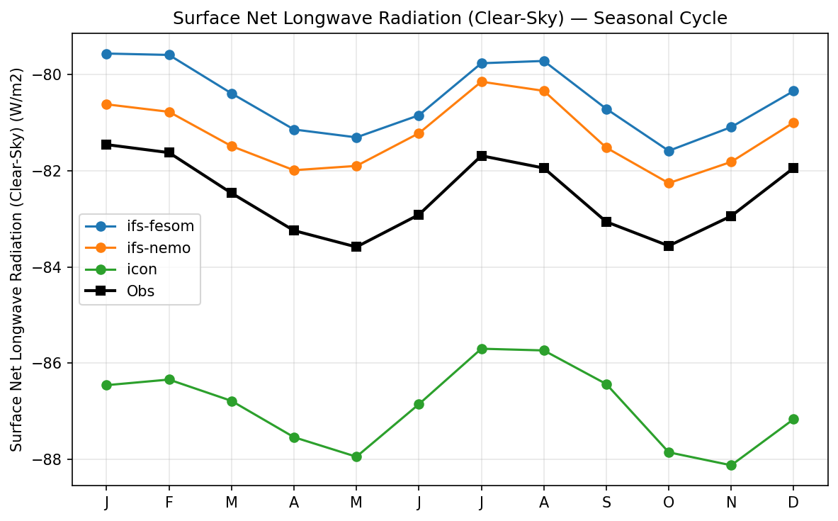
Surface Net Longwave Radiation (Clear-Sky) Seasonal Cycle
| Variables | avg_snlwrfcs |
|---|---|
| Models | ifs-fesom, ifs-nemo, icon |
| Reference Dataset | ERA5 |
| Units | W/m2 |
| Period | 1990–2014 |
Summary high
The figure illustrates the global mean seasonal cycle of clear-sky surface net longwave radiation for three high-resolution models compared to observations (ERA5).
Key Findings
- All models successfully capture the semi-annual structure of the observed global mean seasonal cycle, characterized by strongest net surface cooling in May and October/November.
- The IFS-based models (IFS-FESOM and IFS-NEMO) exhibit a systematic positive bias of 1 to 2 W/m², underestimating the net clear-sky longwave cooling at the surface.
- ICON displays a substantial negative bias of approximately 4 to 5 W/m², heavily overestimating the net clear-sky longwave cooling at the surface.
Spatial Patterns
As a global mean time series, the plot reflects the integrated semi-annual pattern driven by the alternating seasonal cycles of the Northern and Southern Hemispheres. The observed amplitude of the cycle is approximately 2.5 W/m² (ranging from roughly -81.5 to -84 W/m²), a magnitude and phase that all three models reproduce accurately despite their constant mean-state offsets.
Model Agreement
The two IFS-coupled models agree closely with each other, sharing similar phase, amplitude, and a slight positive mean-state bias, which is expected given their shared atmospheric component. ICON diverges significantly in its mean climatology, exhibiting a distinct negative offset, though it maintains excellent agreement with the observed seasonal phase.
Physical Interpretation
Clear-sky surface net longwave radiation is controlled by surface temperature (driving upward emission) and atmospheric temperature and moisture profiles (driving downward emission). The systematic offset in ICON suggests it either has a warmer global mean surface temperature or a drier/cooler lower troposphere than ERA5, leading to enhanced net surface heat loss. Conversely, the IFS models' positive bias implies a slightly cooler surface or a moister/warmer lower atmosphere, increasing downward longwave radiation and dampening net surface cooling.
Caveats
- Global mean seasonal cycles can obscure significant compensating regional biases between the tropics and extratropics.
- Differences in how 'clear-sky' conditions are defined, sampled, and computed in the models' radiative transfer schemes versus the ERA5 assimilation system can introduce artificial biases.
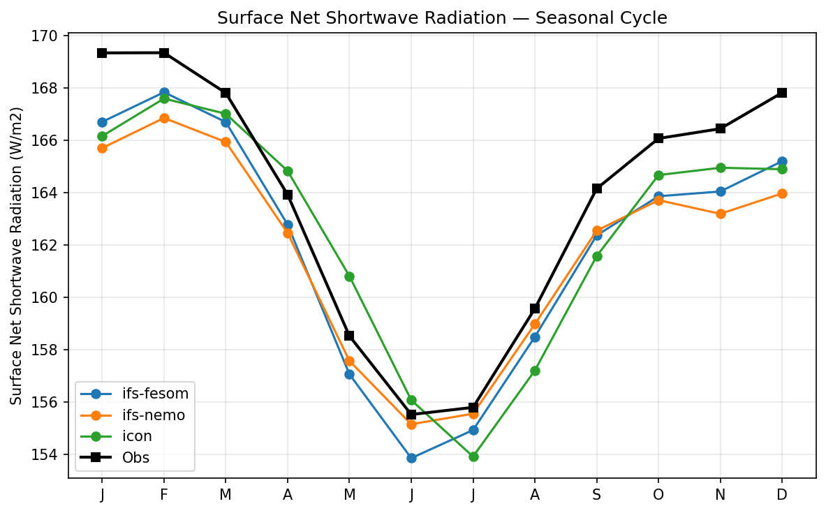
Surface Net Shortwave Radiation Seasonal Cycle
| Variables | avg_snswrf |
|---|---|
| Models | ifs-fesom, ifs-nemo, icon |
| Reference Dataset | ERA5 |
| Units | W/m2 |
| Period | 1990–2014 |
Summary high
The figure displays the monthly climatological cycle of global mean surface net shortwave radiation, showing that all three high-resolution models capture the seasonal phase but systematically underestimate the radiation compared to ERA5, particularly during the boreal winter/austral summer.
Key Findings
- All models exhibit a systematic negative bias of approximately 1-3 W/m2 relative to ERA5 for most of the year.
- The negative bias is most pronounced during the Southern Hemisphere summer (November-March) and minimizes during the Northern Hemisphere summer (June-July).
- Model spread is generally small (~1-2 W/m2), with IFS-FESOM and IFS-NEMO tracking closely, while ICON diverges slightly during the boreal spring and summer.
Spatial Patterns
The temporal pattern shows a global maximum in January/February (~169 W/m2 in observations) and a minimum in June/July (~155-156 W/m2). The models consistently reproduce this seasonal cycle amplitude and phase but are uniformly shifted downward, with the largest model-observation discrepancies occurring from September to March.
Model Agreement
The models exhibit high inter-model agreement, clustering within 1-2 W/m2 of each other throughout the year. However, there is moderate to poor model-observation agreement, as all models fail to reach the magnitude of the ERA5 observations, indicating a shared systemic bias.
Physical Interpretation
The global mean surface net shortwave radiation cycle is driven by Earth's orbital eccentricity (perihelion in January) and hemispheric differences in land fraction and cloud cover. The systematic negative bias, particularly large during the Southern Hemisphere summer (Dec-Feb), strongly suggests that the models simulate overly reflective clouds (too much cloud cover or too high optical depth) or excessive surface albedo (e.g., sea ice) in the Southern Hemisphere. The narrowing of the bias in June/July suggests better representation of Northern Hemisphere summer clouds and land albedo.
Caveats
- ERA5 surface radiation relies on model parameterizations and assimilations, and may itself contain biases compared to direct satellite observations like CERES.
- Global mean time series can mask large compensating regional biases, such as errors in tropical deep convection canceling out errors in Southern Ocean stratocumulus.
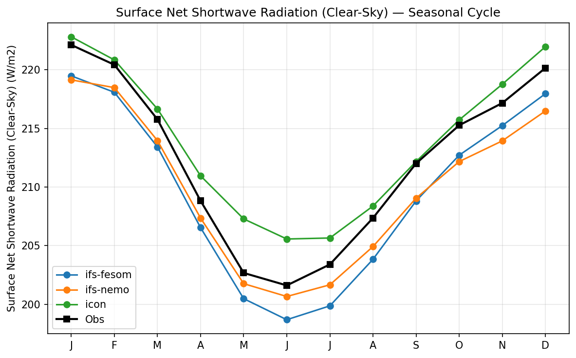
Surface Net Shortwave Radiation (Clear-Sky) Seasonal Cycle
| Variables | avg_snswrfcs |
|---|---|
| Models | ifs-fesom, ifs-nemo, icon |
| Reference Dataset | ERA5 |
| Units | W/m2 |
| Period | 1990–2014 |
Summary high
The figure displays the global mean seasonal cycle of clear-sky surface net shortwave radiation, showing a December-January maximum and a June-July minimum that is broadly captured by all models.
Key Findings
- The ICON model most accurately reproduces the observed ERA5 climatology, exhibiting a very slight positive bias of ~1-2 W/m2 throughout the year.
- Both IFS-based models (IFS-FESOM and IFS-NEMO) systematically underestimate clear-sky surface net shortwave radiation by 2 to 4 W/m2 year-round.
- All models perfectly capture the phase and amplitude of the seasonal cycle, which is governed by orbital parameters and hemispheric asymmetry.
Spatial Patterns
The temporal pattern exhibits a robust global annual cycle peaking in December/January (~222 W/m2) and reaching a minimum in June/July (~201 W/m2). This temporal variation is primarily driven by the Earth's orbital eccentricity (perihelion in January, aphelion in July) combined with hemispheric differences in land fraction, which influences global mean surface albedo and water vapor concentrations.
Model Agreement
There is excellent agreement in phase across all models and observations. Regarding magnitude, ICON demonstrates the highest fidelity. IFS-FESOM and IFS-NEMO agree closely with one another, as expected given their shared IFS atmospheric component, but both feature a persistent negative offset compared to observations. IFS-FESOM yields slightly lower values than IFS-NEMO, particularly during the boreal summer minimum.
Physical Interpretation
Since clear-sky radiation excludes cloud effects, the simulated fluxes are determined by incoming insolation, atmospheric attenuation (scattering and absorption by aerosols, water vapor, and ozone), and surface albedo. The systematic negative bias in the IFS models points to either an overly reflective surface albedo (e.g., over land or sea ice), excessive atmospheric aerosol loading, or excessively high column water vapor compared to ERA5. The minor differences between IFS-FESOM and IFS-NEMO are likely tied to surface albedo differences stemming from their distinct ocean and sea-ice model components.
Caveats
- The global mean diagnostic can obscure large regional compensating biases, such as differences in aerosol loading over industrial regions versus surface albedo biases over polar ice.
- The observational reference (ERA5) is a reanalysis product; its clear-sky radiative fluxes are derived from the assimilating model's radiation scheme rather than direct observations, meaning it carries its own structural uncertainties.
Total Cloud Cover Seasonal Cycle
| Variables | avg_tcc |
|---|---|
| Models | ifs-fesom, ifs-nemo, icon, MPI-ESM1-2-LR, GISS-E2-1-G, IPSL-CM6A-LR, ACCESS-ESM1-5, EC-Earth3, CNRM-CM6-1, AWI-CM-1-1-MR, CNRM-ESM2-1, FGOALS-g3, INM-CM5-0, MRI-ESM2-0 |
| Reference Dataset | ERA5 |
| Units | % |
| Period | 1990–2014 |
Summary high
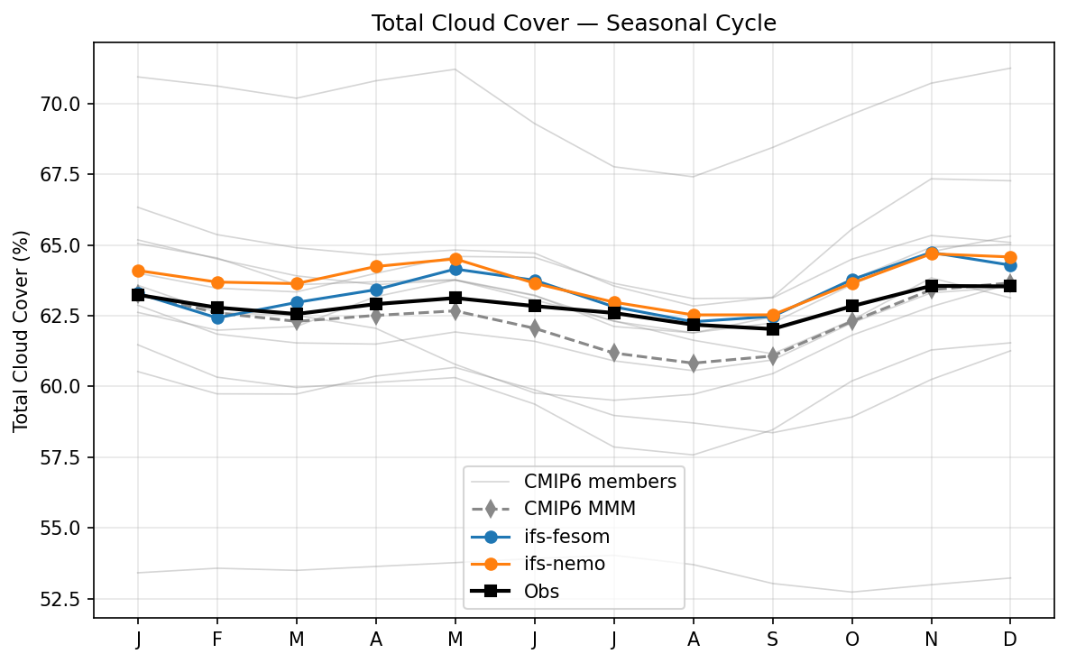
The figure displays the global mean seasonal cycle of Total Cloud Cover (TCC) for high-resolution DestinE models (IFS-FESOM, IFS-NEMO) compared against ERA5 observations and a CMIP6 ensemble.
Key Findings
- IFS-FESOM and IFS-NEMO consistently overestimate global mean Total Cloud Cover compared to ERA5, with biases ranging from +0.5% to +1.5% throughout the year.
- The CMIP6 ensemble exhibits a massive inter-model spread (approx. 53% to 71%), highlighting persistent structural uncertainties in cloud parameterizations in standard-resolution models.
- The two IFS-based models show nearly identical seasonal cycles, indicating that global mean cloud fraction is tightly controlled by the atmospheric component (IFS) and is insensitive to the choice of the coupled ocean model.
Spatial Patterns
Temporally, observed global TCC shows a primary maximum in boreal winter (Nov-Jan, ~63.5%) and a minimum in late boreal summer (Aug-Sep, ~62%). The IFS-based models correctly capture the late-year peak but introduce a spurious, pronounced secondary maximum in boreal spring (May, ~64.5%) that is much weaker in the observations.
Model Agreement
Inter-model agreement between IFS-FESOM and IFS-NEMO is exceptionally high. The CMIP6 ensemble shows very poor inter-model agreement (spread of over 15% in absolute TCC), although the CMIP6 multi-model mean tracks the observed seasonal phase slightly better than the DestinE models, albeit with a slight negative bias.
Physical Interpretation
The vast CMIP6 spread reflects fundamental difficulties in parameterizing sub-grid scale cloud processes (e.g., shallow convection, boundary layer clouds) at ~100 km resolutions. The persistent positive bias and exaggerated spring peak in the high-resolution IFS models likely originate from structural biases within the IFS cloud and convection schemes. The identical behavior of IFS-NEMO and IFS-FESOM confirms that global mean cloudiness is governed by atmospheric physics rather than high-resolution ocean-atmosphere coupling differences.
Caveats
- ERA5 reanalysis is used as the observational reference; reanalysis cloud cover relies heavily on the underlying forecast model and may diverge from direct satellite retrievals (like CERES or ISCCP).
- Global mean time series obscure regional compensating errors, such as potential underestimations of marine stratocumulus canceling out overestimations of storm-track clouds.
TOA Net Longwave Radiation Seasonal Cycle
| Variables | avg_tnlwrf |
|---|---|
| Models | ifs-fesom, ifs-nemo, icon |
| Reference Dataset | ERA5 |
| Units | W/m2 |
| Period | 1990–2014 |
Summary high
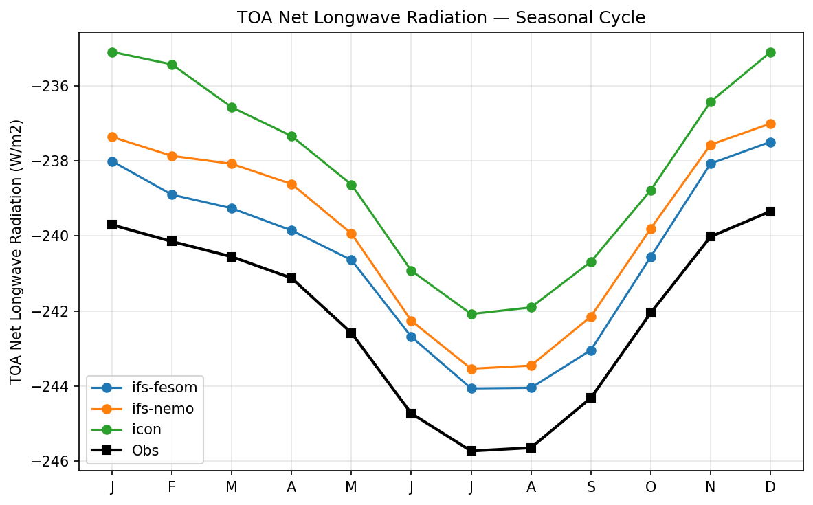
The figure illustrates the global mean seasonal cycle of TOA Net Longwave Radiation, showing that all three high-resolution models accurately reproduce the observed seasonal phase and amplitude but systematically underestimate the magnitude of outgoing longwave radiation.
Key Findings
- All models exhibit a systematic positive bias (less outgoing longwave radiation) ranging from approximately 2 to 5 W/m2 compared to ERA5 observations throughout the year.
- The models successfully capture the seasonal cycle's phase and peak-to-peak amplitude (~6.5 W/m2), with maximum outgoing radiation (most negative) occurring in July-August.
- Among the models, ifs-fesom performs best with the smallest bias (~2 W/m2), followed closely by ifs-nemo, while icon shows the largest discrepancy (~4-5 W/m2) from observations.
Spatial Patterns
The temporal pattern is characterized by a pronounced seasonal cycle with a minimum (highest outgoing radiation, ~-246 W/m2 in observations) during the Northern Hemisphere summer (July-August) and a maximum (lowest outgoing radiation, ~-239.5 W/m2) during the Northern Hemisphere winter (December-January).
Model Agreement
There is strong inter-model agreement regarding the shape, phase, and amplitude of the seasonal cycle. However, all models systematically disagree with observations on the absolute magnitude, consistently simulating insufficient outgoing longwave radiation.
Physical Interpretation
The seasonal cycle itself is driven by the Northern Hemisphere's larger land fraction, which leads to higher global mean surface temperatures and corresponding higher longwave emission during boreal summer. The systematic underestimation of outgoing longwave radiation in the models (positive bias) likely points to either an overestimation of high clouds (which trap outgoing longwave radiation by emitting at colder temperatures) or a widespread cold bias in surface or atmospheric temperatures.
Caveats
- The observational reference used is ERA5 reanalysis, which relies on model physics to derive radiative fluxes and may differ from direct satellite measurements like CERES.
- Global mean time series obscure potential compensating regional biases, such as opposing errors in tropical deep convection and extratropical stratiform clouds.
TOA Net Longwave Radiation (Clear-Sky) Seasonal Cycle
| Variables | avg_tnlwrfcs |
|---|---|
| Models | ifs-fesom, ifs-nemo, icon |
| Reference Dataset | ERA5 |
| Units | W/m2 |
| Period | 1990–2014 |
Summary high
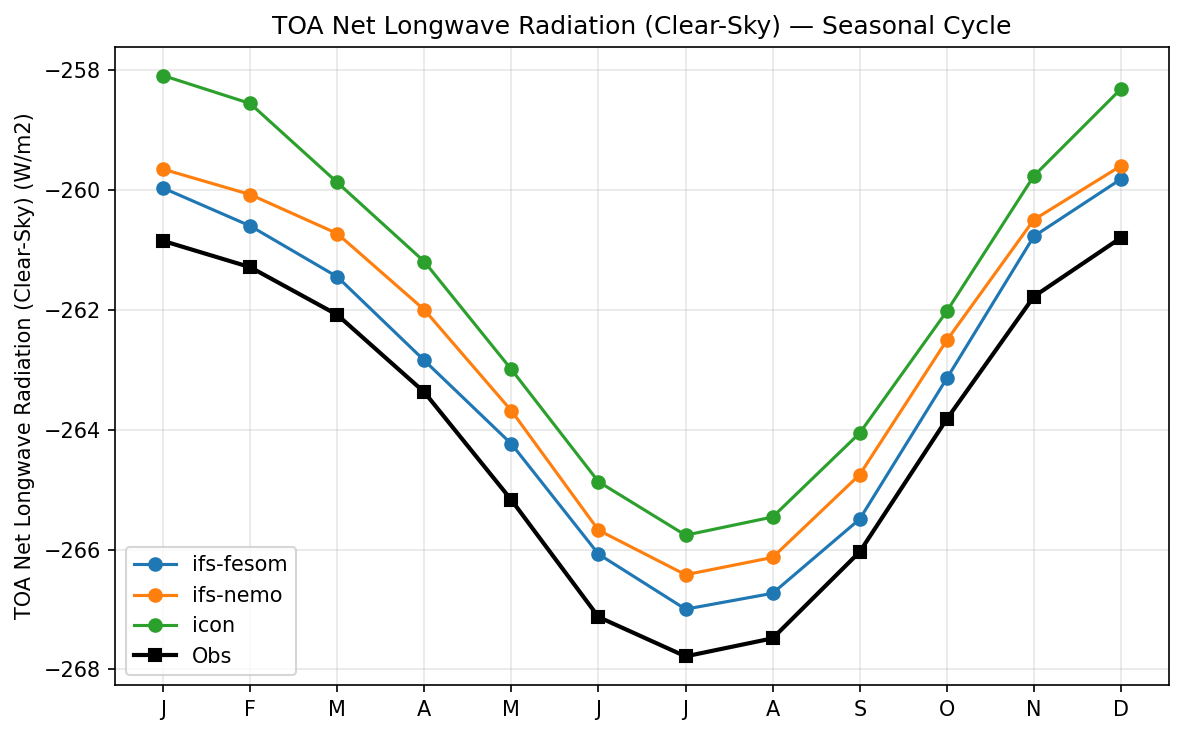
The figure illustrates the global mean seasonal cycle of clear-sky Top-Of-Atmosphere (TOA) Net Longwave Radiation, comparing three high-resolution models against observational data (ERA5).
Key Findings
- All models correctly capture the seasonal phase, with the strongest outgoing radiation (most negative values) in July and the weakest in December/January.
- All models systematically underestimate the magnitude of outgoing clear-sky longwave radiation, exhibiting a positive bias (less negative values) relative to observations throughout the year.
- IFS-FESOM shows the best agreement with observations (bias of ~1 W/m2), followed by IFS-NEMO, while ICON exhibits the largest positive bias (~3-4 W/m2).
Spatial Patterns
The global mean seasonal cycle is dominated by the Northern Hemisphere due to its larger land fraction. Higher surface temperatures during the NH summer (July) lead to increased thermal emission, creating the seasonal minimum (most negative TOA net longwave radiation).
Model Agreement
There is excellent agreement among the models and observations regarding the timing and amplitude of the seasonal cycle. However, inter-model spread is evident in the global mean baseline, with all models showing a systematic positive bias compared to ERA5, ranking from IFS-FESOM (closest) to ICON (furthest).
Physical Interpretation
The systematic underestimation of outgoing clear-sky longwave radiation (positive bias) across all models suggests either a persistent cold surface/tropospheric temperature bias or an overly moist free troposphere, as excessive water vapor would absorb upwelling surface emission and radiate to space at colder, higher altitudes. The accurate representation of the seasonal cycle phase indicates that the models correctly simulate the global hemispheric temperature asymmetry driven by NH landmasses.
Caveats
- The observational reference (ERA5) is a reanalysis, meaning its clear-sky radiative fluxes are model-derived and dependent on the ECMWF radiation scheme rather than direct satellite measurements like CERES.
- Differences in how clear-sky conditions are sampled or defined (e.g., method II vs. method I) between the models and the reanalysis product can introduce artificial biases in clear-sky radiative fluxes.
TOA Net Shortwave Radiation Seasonal Cycle
| Variables | avg_tnswrf |
|---|---|
| Models | ifs-fesom, ifs-nemo, icon |
| Reference Dataset | ERA5 |
| Units | W/m2 |
| Period | 1990–2014 |
Summary high
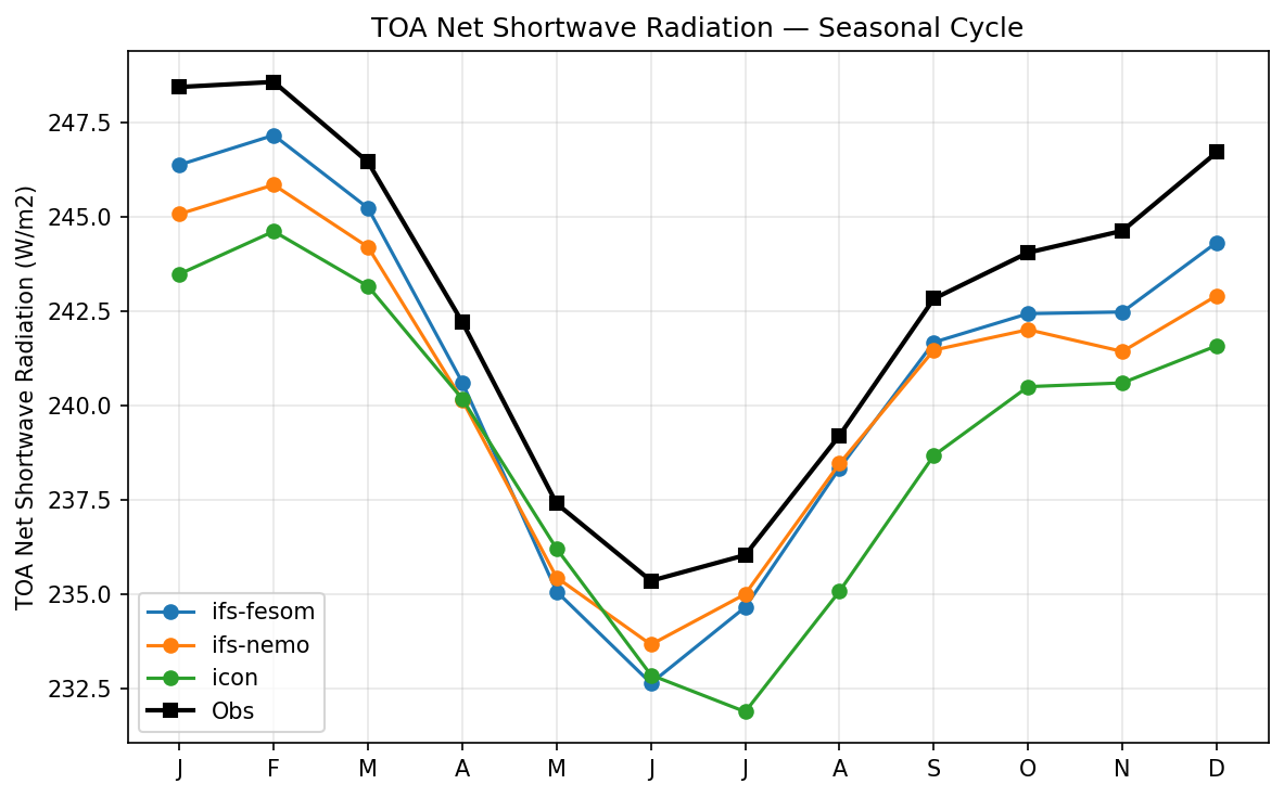
The figure illustrates the seasonal cycle of global mean TOA net shortwave radiation, showing that all three high-resolution models systematically underestimate the observational baseline throughout the year.
Key Findings
- All models correctly capture the phase and amplitude of the seasonal cycle, with a maximum in January/February and a minimum in June/July.
- A systematic negative bias of 1-4 W/m2 is present in all models, indicating that they reflect too much shortwave radiation back to space compared to observations.
- ifs-fesom exhibits the smallest bias, while icon shows the largest negative bias, particularly in the boreal autumn and winter (August-December).
Spatial Patterns
While this is a global mean time series, the prominent seasonal amplitude (~13 W/m2) reflects the combined effects of Earth's orbital eccentricity (perihelion in January) and the hemispheric asymmetry in land/ocean distribution (lower albedo over the Southern Hemisphere ocean during its summer).
Model Agreement
The models show high structural agreement in capturing the seasonal phase. However, there is a consistent inter-model spread of ~1-3 W/m2, with the two IFS-based models grouping closer together and performing better than ICON.
Physical Interpretation
The persistent negative bias in TOA net shortwave radiation implies a planetary albedo that is too high. In climate models, this is most frequently driven by excessive cloud fraction or excessive cloud liquid water/optical depth, particularly in low-level marine stratocumulus regions or over the Southern Ocean.
Caveats
- The observational baseline is ERA5, a reanalysis product that models its own clouds and radiation; comparing against direct satellite measurements like CERES EBAF is recommended for definitive TOA radiation assessments.
- Global mean metrics can mask large compensating regional biases, such as excessive reflection in the tropics compensating for deficient reflection in the high latitudes.
TOA Net Shortwave Radiation (Clear-Sky) Seasonal Cycle
| Variables | avg_tnswrfcs |
|---|---|
| Models | ifs-fesom, ifs-nemo, icon |
| Reference Dataset | ERA5 |
| Units | W/m2 |
| Period | 1990–2014 |
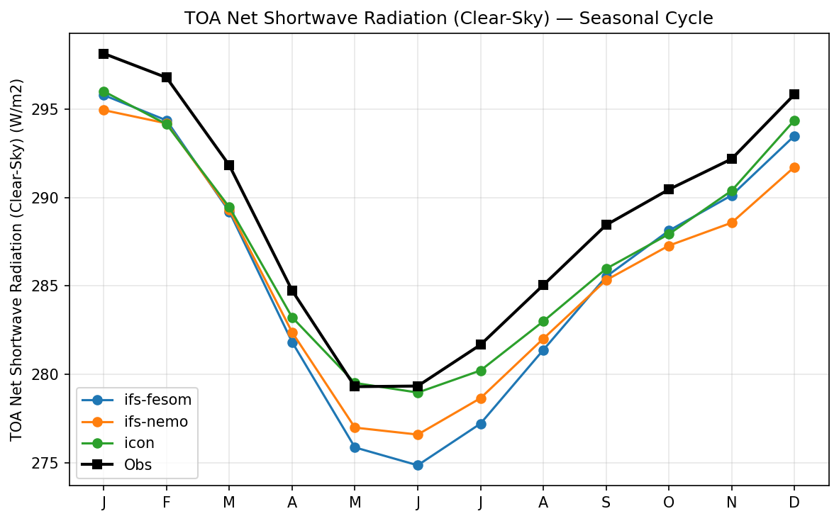
Summary high
The figure displays the monthly climatological seasonal cycle of global mean TOA Net Shortwave Radiation (Clear-Sky) for three high-resolution models compared to observations (ERA5).
Key Findings
- All models correctly capture the phase of the seasonal cycle but systematically underestimate the net clear-sky shortwave radiation at the top of the atmosphere.
- ICON demonstrates the best performance, closely matching observations during the boreal spring and early summer (March-June).
- IFS-FESOM and IFS-NEMO exhibit larger negative biases, especially during boreal summer (May-August), with IFS-FESOM showing the most pronounced underestimation (~4-5 W/m2).
Spatial Patterns
As a global mean diagnostic, spatial patterns are absent. Temporally, the seasonal cycle exhibits a global maximum in December/January (~298 W/m2) and a minimum in June (~279 W/m2), primarily governed by Earth's orbital eccentricity and the seasonal distribution of snow/ice cover and landmass exposure.
Model Agreement
The models agree on the amplitude and phase of the seasonal cycle but differ in absolute magnitude. ICON consistently outperforms the IFS-based models. Notably, IFS-FESOM and IFS-NEMO diverge significantly during boreal summer despite sharing the same atmospheric model.
Physical Interpretation
A systematic negative bias in clear-sky net TOA shortwave radiation indicates that the models reflect too much incoming solar radiation (i.e., the clear-sky planetary albedo is too high). This can be driven by excessive atmospheric scattering (e.g., high aerosol optical depth) or overly reflective surface conditions (e.g., positive biases in sea ice extent, snow cover, or land surface albedo). The notable divergence between IFS-NEMO and IFS-FESOM, which share the same atmosphere, strongly suggests that differences in surface albedo over the ocean—likely tied to sea ice parameterizations or extent—are responsible for the varying biases.
Caveats
- Clear-sky radiative flux diagnostics are highly sensitive to the method used for cloud masking and clear-sky sampling, which can differ between models and observational products.
- The reference dataset is ERA5 (reanalysis) rather than a direct satellite observation product like CERES; reanalysis radiative fluxes are themselves model-derived and subject to biases.
Total Precipitation Rate Seasonal Cycle
| Variables | avg_tprate |
|---|---|
| Models | ifs-fesom, ifs-nemo, icon, MPI-ESM1-2-LR, GISS-E2-1-G, IPSL-CM6A-LR, ACCESS-ESM1-5, EC-Earth3, CNRM-CM6-1, AWI-CM-1-1-MR, CNRM-ESM2-1, FGOALS-g3, INM-CM5-0, MRI-ESM2-0 |
| Reference Dataset | ERA5 |
| Units | kg/m2/s |
| Period | 1990–2014 |
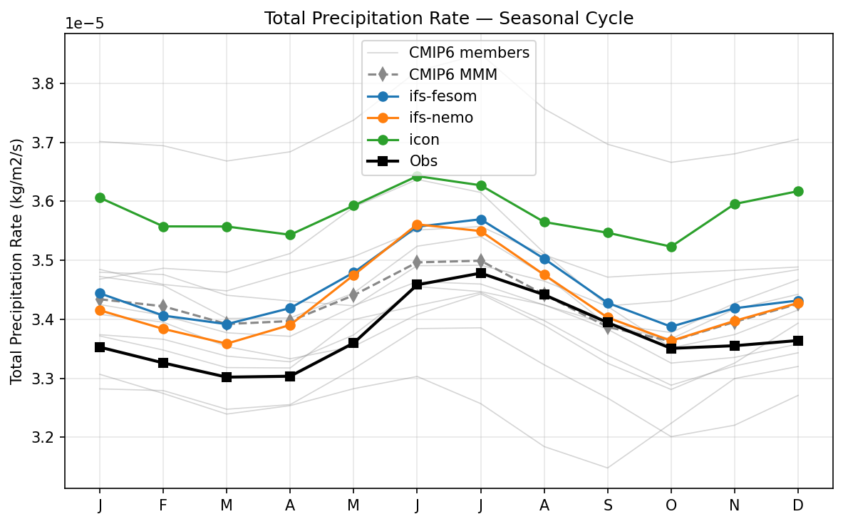
Summary high
The figure illustrates the seasonal cycle of the global mean total precipitation rate, showing that all DestinE high-resolution models reproduce the observed phase but exhibit a consistent positive (wet) bias relative to ERA5.
Key Findings
- All three high-resolution models (IFS-FESOM, IFS-NEMO, ICON) and the CMIP6 multi-model mean successfully capture the bimodal seasonal cycle phase, with a pronounced peak in boreal summer (June-August) and minima in spring and autumn.
- ICON displays a substantial positive bias across all months, sitting near the upper bound of the CMIP6 ensemble spread (~3.6e-5 kg/m2/s).
- IFS-FESOM and IFS-NEMO show excellent mutual agreement and closely track the CMIP6 multi-model mean, exhibiting a more moderate wet bias compared to ERA5.
Spatial Patterns
As a global mean time series, spatial patterns are averaged out. Temporally, the observed seasonal amplitude (difference between July peak and March minimum) is roughly 0.18e-5 kg/m2/s. The DestinE models exhibit similar or slightly amplified seasonal amplitudes, maintaining their respective positive offsets year-round.
Model Agreement
Inter-model agreement is very high between IFS-FESOM and IFS-NEMO, which track almost identically. ICON diverges significantly with a systematic upward shift. None of the DestinE models perfectly match the absolute magnitude of the ERA5 observations, though they fall within the broad spread of the CMIP6 ensemble.
Physical Interpretation
The boreal summer peak in global precipitation is driven by the northward shift of the ITCZ and the activation of Northern Hemisphere monsoons over large land masses. The systematic wet bias in the high-resolution models, particularly ICON, may stem from overly active convective parameterizations or differences in cloud microphysics at the ~5 km 'grey zone' resolution, which often leads to intensified global hydrological cycles compared to reanalyses.
Caveats
- Global mean precipitation masks large regional compensating errors (e.g., overly intense ITCZ vs. excessively dry subtropics).
- Precipitation in ERA5 is a forecasted field rather than a directly assimilated observation; evaluating against satellite-gauge products (e.g., GPCP) is necessary to confirm the absolute magnitude of the model biases.