Ocean 3d Ocean Evaluation (EN4)
Synthesis
Related diagnostics
Salinity Depth-Layer Time Series
| Variables | avg_thetao, avg_so |
|---|---|
| Models | ifs-fesom, ifs-nemo, icon, EN4 |
| Reference Dataset | EN4 v4.2.2 |
| Units | K |
| Period | 1990–2014 |
Summary high
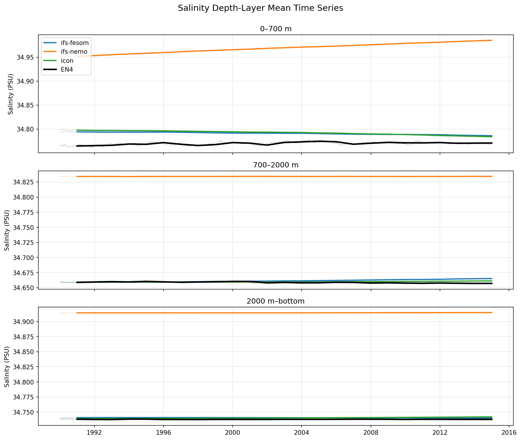
Time series of volume-weighted mean global salinity across three depth layers (0-700 m, 700-2000 m, 2000 m-bottom), comparing three high-resolution models against EN4 observational data from 1990 to 2015.
Key Findings
- IFS-NEMO exhibits a massive, systematic salty bias of approximately +0.17 to +0.18 PSU across all depth layers from the start of the simulation.
- IFS-FESOM and ICON show a progressive freshening drift in the upper ocean (0-700 m) over the 25-year period, diverging from the relatively stable EN4 observations.
- In the deep ocean (2000 m-bottom), IFS-FESOM and ICON accurately capture the absolute salinity and exhibit minimal drift, matching EN4 closely.
Spatial Patterns
The upper ocean (0-700 m) shows a continuous freshening trend for both IFS-FESOM and ICON. In the intermediate layer (700-2000 m), IFS-FESOM shows a slight salinification drift while ICON shows a minor freshening drift. The deep ocean remains stable across all models, reflecting the long timescales required for deep water mass ventilation.
Model Agreement
IFS-FESOM and ICON generally agree with each other and with EN4 in the deep ocean, but diverge from observations in the upper ocean due to long-term drift. IFS-NEMO is an extreme outlier, failing to agree with observations or the other models at any depth due to a severe initial offset.
Physical Interpretation
The extreme and immediate salty bias in IFS-NEMO across all depths strongly indicates an error in the initial conditions, such as using a different reference salinity or an incorrect initialization file. The steady freshening drift in the upper 700 m for IFS-FESOM and ICON suggests a global freshwater imbalance, potentially driven by excess precipitation over evaporation (P-E bias), excessive continental runoff, or overly rapid sea ice melt in the coupled system.
Caveats
- EN4 observational data has high uncertainty in the deep ocean (below 2000 m) due to sparse spatial and temporal sampling prior to the Argo era and the deployment of Deep Argo.
- The 25-year time series is too short to fully evaluate deep ocean drift, which typically operates on centennial to millennial timescales.
Salinity Hovmoller (first-timestep anomaly)
| Variables | avg_thetao, avg_so |
|---|---|
| Models | ifs-fesom, ifs-nemo, icon |
| Reference Dataset | EN4 v4.2.2 |
| Units | K |
| Period | 1990–2014 |
Summary high
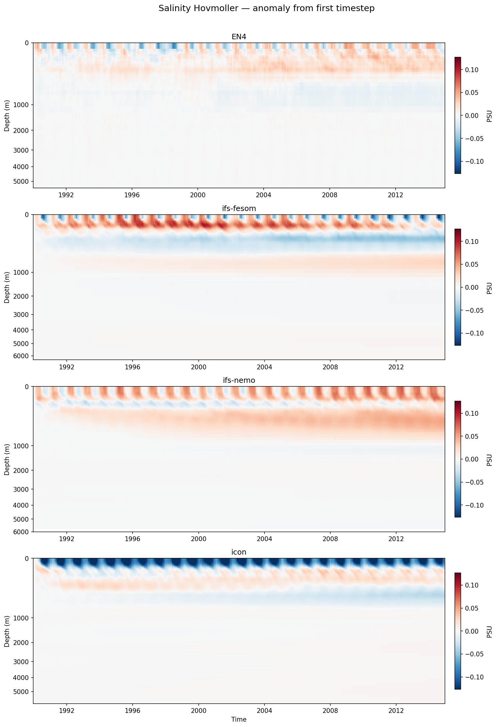
Hovmoller diagram of global mean salinity anomalies relative to the first timestep, illustrating the intrinsic multi-decadal drift of the models compared to EN4 observations over the 1990-2014 period.
Key Findings
- All models exhibit significant intrinsic salinity drift in the upper 1500m, with magnitudes exceeding the observational trends in EN4.
- ICON shows a pronounced and progressive surface freshening trend, directly contradicting the surface salinification observed in EN4 and simulated by the IFS models.
- The vertical structure of subsurface salinity drift varies fundamentally between the models, indicating different biases in vertical mixing and intermediate water formation.
Spatial Patterns
Drift signals are predominantly confined to the upper 1500m. EN4 shows mild surface salinification and slight subsurface freshening (200-1000m). IFS-FESOM exaggerates this pattern with intense surface salinification and a strong freshening layer at 200-600m. IFS-NEMO develops a thick, deepening salinification layer between 400-1000m. ICON displays an inverted profile with intense surface freshening (0-200m) and subsurface salinification (200-600m).
Model Agreement
Models agree on the presence of a strong seasonal cycle in the upper ~100m, but inter-model agreement on long-term trends and vertical anomaly structure is very poor. None of the models accurately reproduce the relatively stable EN4 observational baseline.
Physical Interpretation
Global mean salinity drift is primarily driven by imbalances in surface freshwater fluxes (Precipitation - Evaporation + Runoff) and deficiencies in vertical mixing or advection. ICON's strong surface freshening suggests an overly positive global freshwater flux into the ocean. The diverse subsurface anomalies, such as IFS-NEMO's 400-1000m salinification, likely result from biases in the subduction and propagation of intermediate water masses.
Caveats
- Global mean vertical profiles can mask large, compensating regional biases (e.g., intense Atlantic salinification compensating for Pacific freshening).
- Anomalies relative to the first timestep reflect intrinsic drift, making the analysis highly sensitive to the initial ocean state in 1990 and the lack of a long spin-up period.
Salinity Hovmoller (EN4-ref anomaly)
| Variables | avg_thetao, avg_so |
|---|---|
| Models | ifs-fesom, ifs-nemo, icon |
| Reference Dataset | EN4 v4.2.2 |
| Units | K |
| Period | 1990–2014 |
Summary high
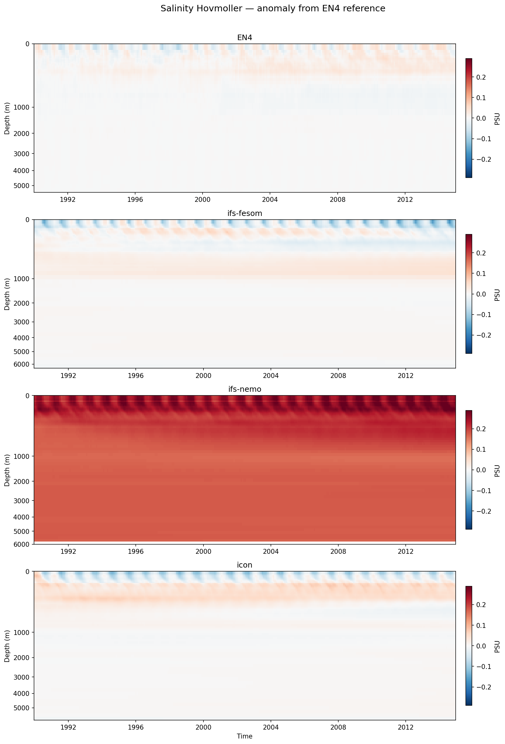
Time-depth Hovmoller diagram of global-mean salinity anomalies relative to the EN4 observational reference profile, showing the evolution of vertical salinity structure from 1990 to 2014.
Key Findings
- ifs-nemo exhibits a severe, pervasive salty bias across the entire water column (>0.2 PSU in the upper 1000m) that is present from the very start of the simulation.
- ifs-fesom and icon show similar anomaly structures, featuring strong surface seasonal cycles, subsurface salty anomalies (between 200-1000m), and relatively stable deep oceans.
- All three models overestimate the amplitude of the surface seasonal salinity cycle compared to EN4 observations.
Spatial Patterns
A pronounced alternating fresh/salty seasonal cycle is visible in the upper ~50m for all models. ifs-fesom develops a fresh anomaly at ~200-500m and a salty anomaly at ~500-1200m. icon shows a salty anomaly peaking around 400-800m. ifs-nemo displays a uniform, deep-reaching salty bias that extends from the surface down to 6000m.
Model Agreement
ifs-fesom and icon agree moderately well with each other in terms of drift magnitude and stable deep oceans, though the exact depth of their subsurface biases differ. ifs-nemo completely diverges from EN4 and the other models due to its massive positive offset.
Physical Interpretation
The immediate, whole-column salty anomaly in ifs-nemo strongly indicates an initialization error or the use of a spin-up state/climatology that is fundamentally much saltier than the EN4 1990 reference, rather than a dynamic model drift. The subsurface salty biases in ifs-fesom and icon likely stem from biases in intermediate water mass formation, subduction rates, or insufficient vertical mixing across the halocline. The overestimated surface seasonality is likely tied to biases in P-E (precipitation minus evaporation) surface fluxes or excessive sea ice melt/freeze cycles.
Caveats
- The massive initial offset in ifs-nemo saturates the color scale and obscures any underlying temporal drift in that model.
- Global mean profiles can mask large, compensating regional biases (e.g., an overly salty Atlantic compensating for a too-fresh Pacific).
- The depth axis is non-linear (likely square-root scaled), which visually exaggerates upper ocean features relative to the deep ocean.
Salinity Surface Annual Mean Bias
| Variables | avg_thetao, avg_so |
|---|---|
| Models | ifs-fesom, ifs-nemo, icon |
| Reference Dataset | EN4 v4.2.2 |
| Units | K |
| Period | 1990–2014 |
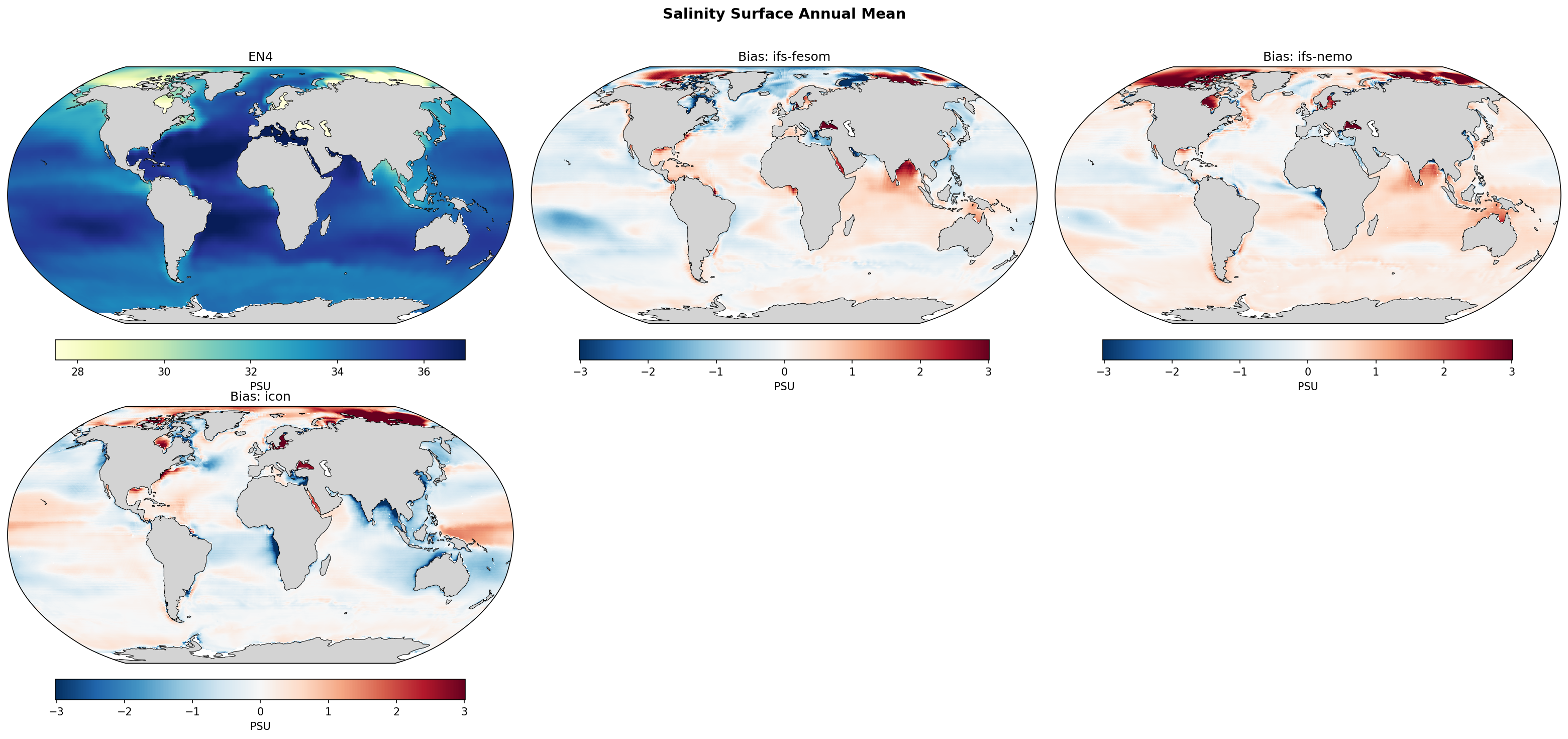
| ifs-fesom | Global Mean Bias: -0.05 · Rmse: 0.67 |
| ifs-nemo | Global Mean Bias: 0.22 · Rmse: 0.73 |
| icon | Global Mean Bias: -0.10 · Rmse: 0.91 |
Summary high
Spatial maps of annual mean sea surface salinity (SSS) climatology biases reveal significant high-latitude and marginal sea errors across all models, with diverging basin-scale biases in the open ocean.
Key Findings
- All models exhibit extreme SSS biases (exceeding ±3 PSU) in the Arctic Ocean and marginal seas such as the Baltic, Mediterranean, and Red Sea.
- IFS-NEMO exhibits a pervasive, systematic salty bias across most global ocean basins (global mean bias +0.218 PSU).
- IFS-FESOM has the lowest overall error (RMSE 0.665 PSU) but features a broad fresh bias in the Pacific Ocean and a salty bias in the Indian Ocean.
- ICON shows the highest spatial variance in error (RMSE 0.911 PSU), characterized by strong salty biases in the Arctic and Atlantic, and stark fresh biases in the Indian Ocean (Bay of Bengal) and along western boundary currents.
Spatial Patterns
Extreme biases are concentrated in regions dominated by cryospheric processes (Arctic), enclosed basins with high evaporation (Mediterranean, Red Sea), and areas with massive riverine input (Bay of Bengal, Amazon plume). In the open ocean, large-scale zonal and basin-wide patterns emerge: IFS-FESOM is broadly fresh in the Pacific and salty in the Atlantic/Indian; IFS-NEMO is weakly salty everywhere; ICON shows stark contrasts, such as a fresh Indian Ocean versus a salty Atlantic.
Model Agreement
The models broadly agree on the locations of maximum difficulty (Arctic, marginal seas, river plumes) but disagree substantially on the sign and magnitude of open-ocean basin biases. For example, the Indian Ocean is distinctly fresh in ICON but salty in IFS-FESOM and IFS-NEMO.
Physical Interpretation
Surface salinity is a direct integrator of the freshwater cycle (Evaporation minus Precipitation, E-P), river runoff, and sea ice dynamics. The severe Arctic biases (especially the salty biases in NEMO and ICON) likely stem from inadequate river runoff routing, excessive sea ice formation (brine rejection), or over-mixing with salty subsurface waters. Marginal sea errors highlight challenges in capturing E-P balances and resolving narrow straits (e.g., Strait of Gibraltar) even at high resolutions. Open ocean differences are primarily driven by variations in the atmospheric models' precipitation patterns (e.g., ITCZ positioning) and evaporation rates.
Caveats
- Observational SSS data (EN4) in the Arctic and ice-covered regions has high uncertainty due to sparse in-situ sampling and satellite limitations, meaning model 'biases' here may partially reflect observational gaps.
- Coastal and river plume biases are highly sensitive to how river runoff is routed and distributed in the respective model grids, which may differ significantly from reality.
Salinity Surface DJF Bias

| Variables | avg_thetao, avg_so |
|---|---|
| Models | ifs-fesom, ifs-nemo, icon |
| Reference Dataset | EN4 v4.2.2 |
| Units | K |
| Period | 1990–2014 |
| ifs-fesom | Global Mean Bias: -0.05 · Rmse: 0.69 |
| ifs-nemo | Global Mean Bias: 0.20 · Rmse: 0.73 |
| icon | Global Mean Bias: -0.08 · Rmse: 0.93 |
Summary high
The figure compares the DJF sea surface salinity (SSS) climatology of three high-resolution models (IFS-FESOM, IFS-NEMO, ICON) against EN4 observations, revealing prominent biases in the Arctic, marginal seas, and tropical precipitation zones.
Key Findings
- IFS-NEMO exhibits a widespread, systematic salty bias globally (+0.20 PSU), whereas IFS-FESOM and ICON have slight global fresh biases but larger regional compensations.
- ICON shows the largest overall errors (RMSE 0.93 PSU), driven by severe salty biases in the Arctic and widespread fresh biases in the tropical Indo-Pacific and subpolar North Atlantic.
- All models struggle with salinity in marginal seas (Mediterranean, Red Sea) and the Arctic Ocean, highlighting challenges in representing river runoff, sea ice freshwater fluxes, and strait exchanges.
Spatial Patterns
In the Arctic, ICON and IFS-FESOM show intense salty biases along the Eurasian coast, while IFS-NEMO shows strong salty biases in the Barents and Kara seas. In the tropics, IFS-FESOM and ICON display fresh biases corresponding to the ITCZ and SPCZ. The Mediterranean and Red Seas are consistently too salty across all models. IFS-FESOM and ICON also show notable fresh biases in the subpolar North Atlantic.
Model Agreement
Models disagree significantly on the sign and spatial distribution of global biases. IFS-NEMO is anomalously salty over most open ocean basins. IFS-FESOM and ICON share similar fresh biases in the tropical Pacific and subpolar North Atlantic but diverge in the Indian Ocean. All models agree on the presence of strong salty biases in highly evaporative marginal seas like the Mediterranean.
Physical Interpretation
Arctic and coastal salinity biases are strongly influenced by inaccuracies in river runoff routing, discharge volumes, and sea ice thermodynamic processes (brine rejection and meltwater release). Tropical fresh biases in IFS-FESOM and ICON align with regions of deep convection (ITCZ/SPCZ), suggesting excessive precipitation (P-E deficits) from the atmospheric component. Salty biases in the Mediterranean and Red Sea indicate either excessive evaporation or insufficient freshwater exchange through narrow straits.
Caveats
- EN4 observational data has very high uncertainty in the Arctic Ocean and under sea ice due to extremely sparse historical sampling.
- The metadata specifies units of 'K', which is incorrect; the maps display Practical Salinity Units (PSU).
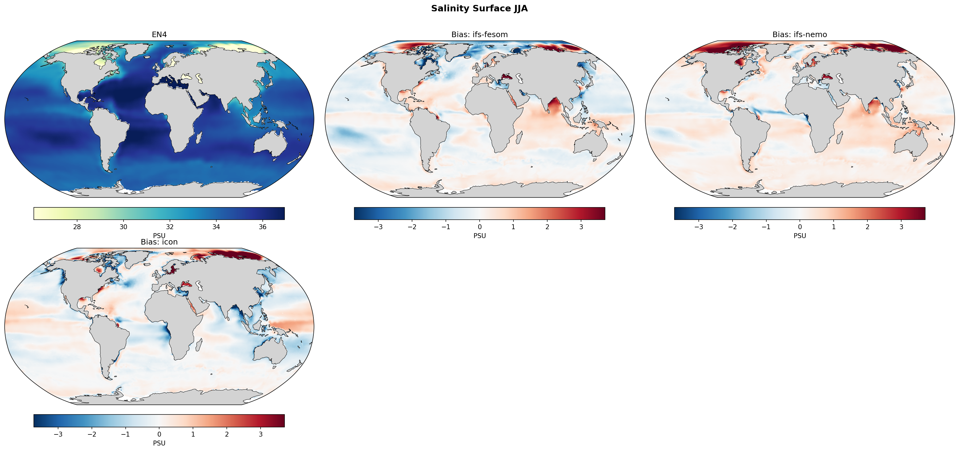
Salinity Surface JJA Bias
| Variables | avg_thetao, avg_so |
|---|---|
| Models | ifs-fesom, ifs-nemo, icon |
| Reference Dataset | EN4 v4.2.2 |
| Units | K |
| Period | 1990–2014 |
| ifs-fesom | Global Mean Bias: -0.06 · Rmse: 0.77 |
| ifs-nemo | Global Mean Bias: 0.24 · Rmse: 0.86 |
| icon | Global Mean Bias: -0.11 · Rmse: 1.00 |
Summary high
The figure displays the June-July-August (JJA) sea surface salinity climatology from the EN4 observational dataset and the corresponding biases for three high-resolution coupled models (IFS-FESOM, IFS-NEMO, ICON).
Key Findings
- All three models exhibit a severe positive (salty) bias in the Arctic Ocean during the JJA season, often exceeding 3 PSU.
- IFS-FESOM demonstrates the best overall performance with the lowest RMSE (0.77 PSU) and a small global mean fresh bias, characterized by broad but moderate fresh anomalies in the Pacific.
- IFS-NEMO shows a systematic global positive bias (+0.24 PSU), being too salty across most open ocean basins, while ICON exhibits the highest RMSE (1.00 PSU) with large regional compensations.
Spatial Patterns
The most prominent shared pattern is the extreme salty anomaly in the Arctic Ocean. In the open ocean, IFS-FESOM displays widespread fresh biases in the North Pacific, tropical Pacific, and North Atlantic. IFS-NEMO shows a contrasting pattern of widespread salty biases across the Pacific, Atlantic, and Indian Oceans. ICON features a distinct dipole in the Pacific, with fresh biases in the North Pacific and strong salty biases in the South Pacific and along the eastern equatorial Pacific. Significant localized biases are evident near major river outflows (e.g., Amazon, Congo) and in marginal seas (e.g., Baltic Sea, Bay of Bengal).
Model Agreement
Models show strong agreement regarding the sign and magnitude of the salty bias in the Arctic. However, they diverge significantly in the open ocean basins, lacking consensus on the sign of the Evaporation minus Precipitation (E-P) driven biases. There is also considerable inter-model disagreement in coastal and marginal sea regions, reflecting differences in how river runoff is handled.
Physical Interpretation
The ubiquitous Arctic salty bias during the JJA melt season is strongly indicative of deficient freshwater input from summer sea ice melt, or potentially underestimated river discharge from high-latitude catchments. Basin-scale biases in the mid-to-low latitudes are primarily driven by errors in the surface freshwater flux (E-P balance); for example, IFS-NEMO's pervasive salty bias suggests excessive evaporation or deficient precipitation globally. Localized extreme biases, such as the salty bias in the Bay of Bengal for IFS-FESOM, highlight challenges in accurately representing intense monsoonal precipitation and river routing, even at ~5 km resolution.
Caveats
- In-situ salinity observations in the EN4 dataset are historically sparse in the Arctic Ocean and under sea ice, meaning the reference climatology has higher uncertainty in the exact region where models show the largest biases.
- Biases in coastal regions and near major estuaries are highly sensitive to the specific river runoff datasets and routing schemes prescribed in the models, which may obscure underlying coupled model physics.
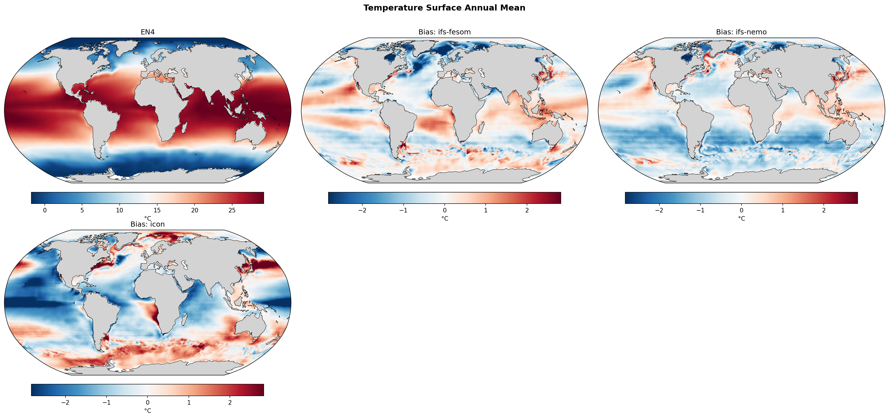
Temperature Surface Annual Mean Bias
| Variables | avg_thetao, avg_so |
|---|---|
| Models | ifs-fesom, ifs-nemo, icon |
| Reference Dataset | EN4 v4.2.2 |
| Units | K |
| Period | 1990–2014 |
| ifs-fesom | Global Mean Bias: 0.00 · Rmse: 0.85 |
| ifs-nemo | Global Mean Bias: -0.35 · Rmse: 0.84 |
| icon | Global Mean Bias: -0.43 · Rmse: 1.41 |
Summary high
The figure displays the annual mean sea surface temperature (SST) climatology from EN4 observations alongside the spatial bias patterns for three high-resolution models: IFS-FESOM, IFS-NEMO, and ICON.
Key Findings
- IFS-FESOM achieves a near-zero global mean SST bias (0.001 K) with an RMSE of 0.85 K, though it relies on compensating regional biases.
- IFS-NEMO exhibits a pervasive cold bias across most ocean basins (global mean -0.35 K) but maintains a low RMSE (0.84 K) comparable to IFS-FESOM.
- ICON demonstrates the largest errors (RMSE 1.41 K, bias -0.43 K), characterized by severe cold biases in the tropics and Northern Hemisphere, contrasted with intense warm biases in the Southern Ocean.
Spatial Patterns
IFS-FESOM shows a warm bias in the eastern tropical Pacific (typical of stratocumulus deficits) and a cold bias in the North Atlantic subpolar gyre. IFS-NEMO displays broad subtropical cold biases but distinct warm biases along the Gulf Stream and Kuroshio extensions. ICON exhibits a stark meridional contrast: severe cold biases throughout the tropics and Northern Hemisphere, paired with intense warm biases across the Southern Ocean and western boundary currents.
Model Agreement
The models diverge significantly in their spatial bias signatures. IFS-FESOM and IFS-NEMO perform similarly well in terms of overall spatial variance (RMSE ~0.84-0.85 K), while ICON struggles significantly more. All three models show varying degrees of warm biases in western boundary current regions (Gulf Stream, Kuroshio, Agulhas), indicating shared challenges in mesoscale ocean dynamics.
Physical Interpretation
The eastern Pacific warm bias in IFS-FESOM is likely linked to underrepresented marine stratocumulus clouds, leading to excessive surface shortwave heating. ICON's massive Southern Ocean warm bias is a classic coupled model error, typically driven by deficits in Southern Ocean cloud cover (too little supercooled liquid water) or inaccurate mixed layer depths. The persistent western boundary current biases across all models suggest that even at ~5 km resolution, capturing the precise separation latitude and eddy-driven heat transport of currents like the Gulf Stream remains difficult.
Caveats
- EN4 is an objective analysis product; data sparsity in the Southern Ocean and polar regions introduces observational uncertainty.
- The 1990-2014 period includes internal decadal variability; uninitialized coupled models will not reproduce the observed phase of modes like the PDO or AMO, which can alias into the climatological bias.
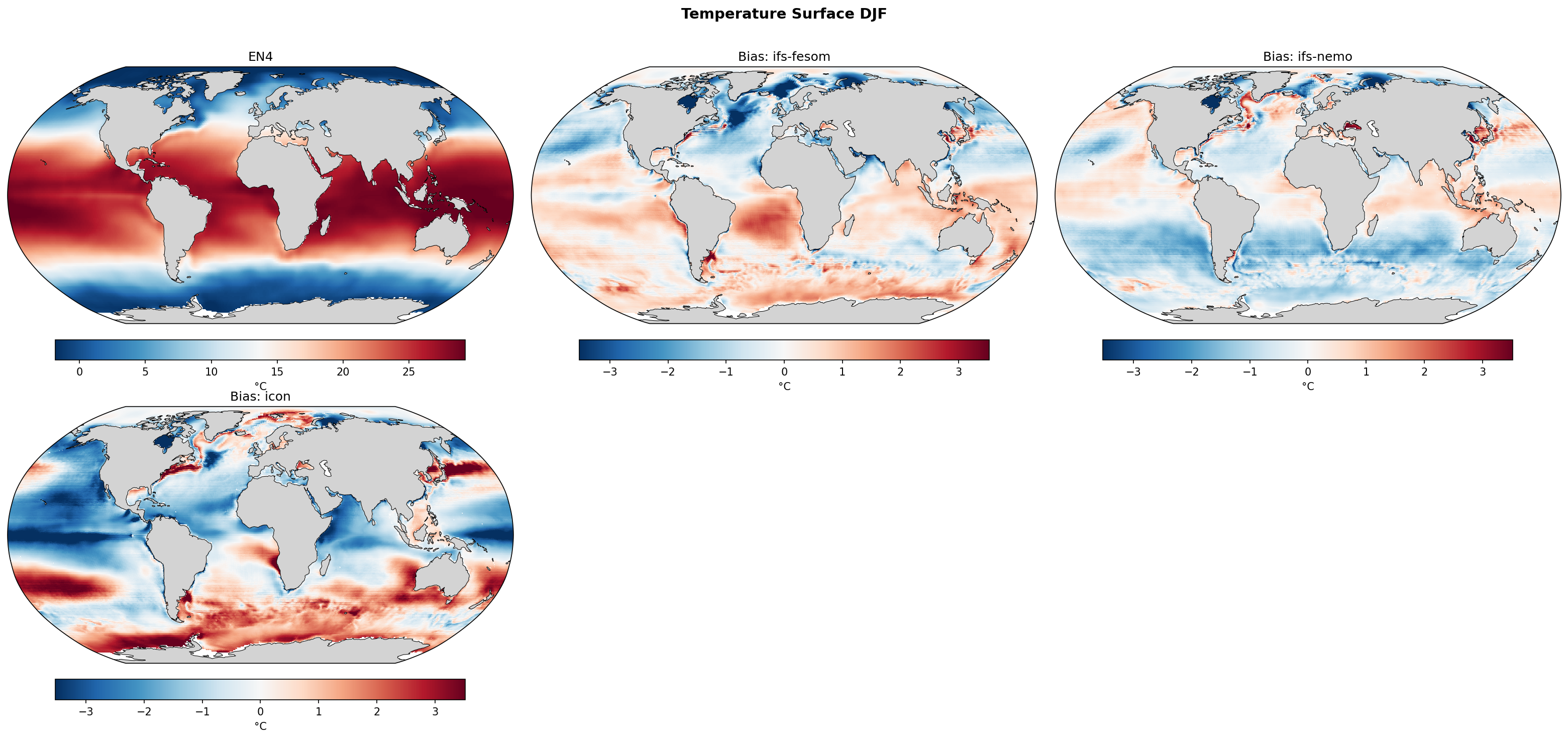
Temperature Surface DJF Bias
| Variables | avg_thetao, avg_so |
|---|---|
| Models | ifs-fesom, ifs-nemo, icon |
| Reference Dataset | EN4 v4.2.2 |
| Units | K |
| Period | 1990–2014 |
| ifs-fesom | Global Mean Bias: 0.09 · Rmse: 1.07 |
| ifs-nemo | Global Mean Bias: -0.35 · Rmse: 0.95 |
| icon | Global Mean Bias: -0.35 · Rmse: 1.79 |
Summary high
This figure displays the December-January-February (DJF) mean Sea Surface Temperature (SST) from EN4 observations and the corresponding bias maps for three high-resolution coupled models (IFS-FESOM, IFS-NEMO, and ICON).
Key Findings
- IFS-NEMO exhibits the lowest overall error (RMSE = 0.95 K), despite a global mean cold bias (-0.35 K) largely driven by the tropical and subtropical oceans.
- ICON shows the most severe spatial biases (RMSE = 1.79 K), characterized by intense tropical cold biases and massive warm biases in the Southern Ocean and North Pacific.
- IFS-FESOM has a near-zero global mean bias (+0.09 K) but displays compensating regional errors, such as a warm bias in the eastern tropical Pacific and Southern Ocean, and a cold bias in the North Atlantic subpolar gyre.
Spatial Patterns
In the tropics, ICON and IFS-NEMO feature a pronounced cold tongue bias extending across the Pacific, Atlantic, and Indian Oceans, whereas IFS-FESOM shows a warm bias in the eastern equatorial Pacific. In the North Atlantic, all models struggle: IFS-FESOM and ICON exhibit strong cold biases in the subpolar gyre, while IFS-NEMO shows a warm bias along the North American coast and Gulf Stream extension. The Southern Ocean exhibits broad warm biases in ICON and IFS-FESOM, which are largely absent or less systematic in IFS-NEMO.
Model Agreement
The models diverge significantly in their regional bias patterns, particularly in the tropical Pacific (warm in FESOM, cold in NEMO/ICON) and the Southern Ocean (strongly warm in ICON, moderately warm in FESOM, mixed in NEMO). However, all models demonstrate elevated errors in regions characterized by strong western boundary currents, such as the Gulf Stream and Kuroshio.
Physical Interpretation
The pervasive cold tropical biases in NEMO and ICON suggest excessively strong trade winds leading to overactive equatorial upwelling. The North Atlantic biases are classic signatures of Gulf Stream separation errors and misrepresentation of the North Atlantic Current pathway, a persistent challenge even at ~5 km resolution. The severe Southern Ocean warm biases, particularly in ICON, frequently stem from insufficient supercooled liquid water in low-level clouds, which leads to excessive surface shortwave absorption.
Caveats
- The analysis is restricted to the DJF season; biases may look different in the annual mean or during the austral winter (JJA).
- Observational uncertainty in EN4 is higher in sparsely sampled regions like the Southern Ocean and near sea-ice margins, which may affect the apparent model biases in these areas.
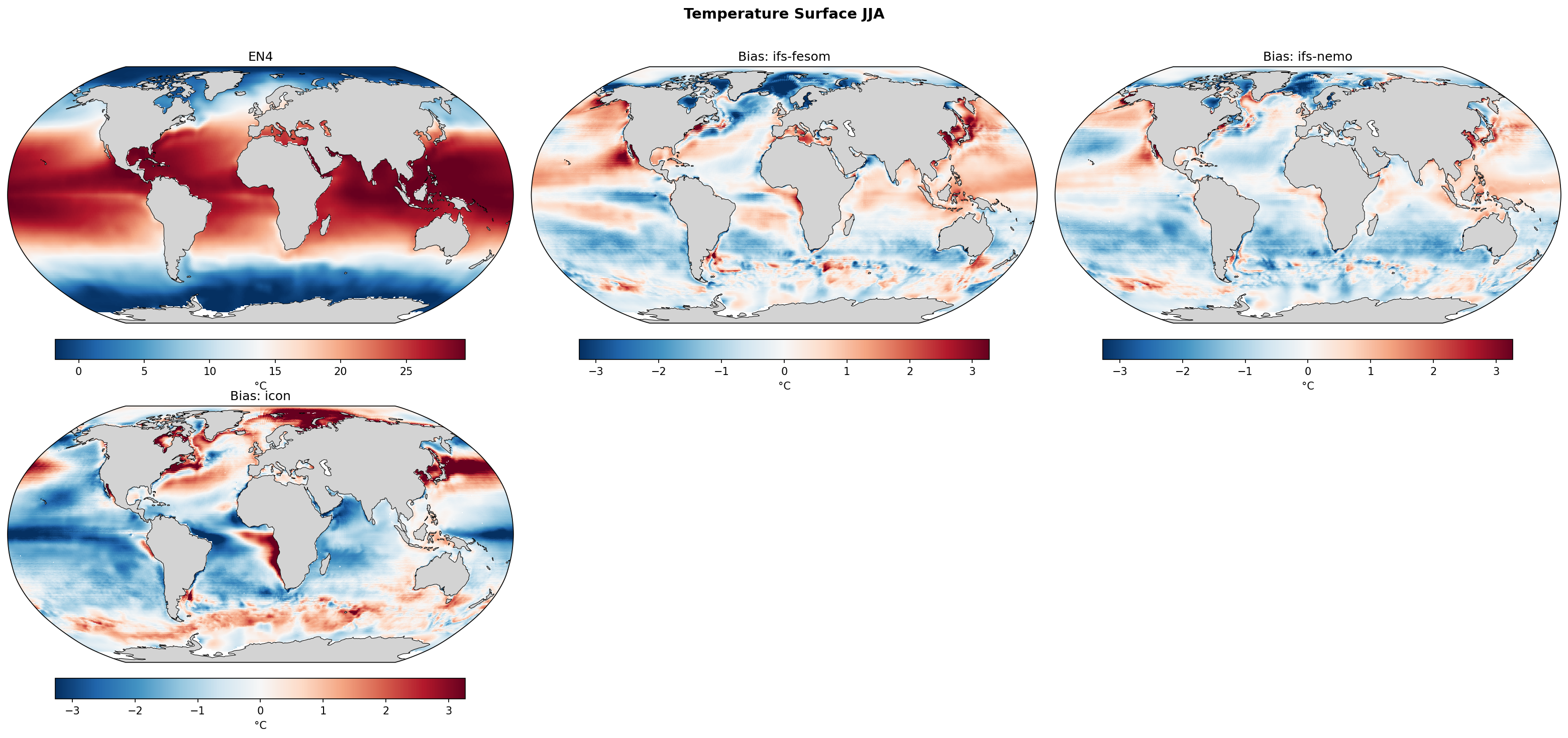
Temperature Surface JJA Bias
| Variables | avg_thetao, avg_so |
|---|---|
| Models | ifs-fesom, ifs-nemo, icon |
| Reference Dataset | EN4 v4.2.2 |
| Units | K |
| Period | 1990–2014 |
| ifs-fesom | Global Mean Bias: -0.08 · Rmse: 1.06 |
| ifs-nemo | Global Mean Bias: -0.35 · Rmse: 0.90 |
| icon | Global Mean Bias: -0.48 · Rmse: 1.49 |
Summary high
This figure displays the global June-July-August (JJA) sea surface temperature (SST) climatology from the EN4 observational dataset alongside spatial bias maps for three high-resolution models (IFS-FESOM, IFS-NEMO, ICON). All models exhibit widespread cold biases, with ICON showing the largest global mean cold bias and RMSE.
Key Findings
- All three models exhibit a global mean cold bias in JJA SST, ranging from -0.08 K (IFS-FESOM) to -0.48 K (ICON).
- ICON displays the largest RMSE (1.49 K) and most pronounced regional biases, particularly in the North Atlantic, North Pacific, and eastern boundary upwelling regions.
- IFS-NEMO has the lowest RMSE (0.90 K) and generally smaller magnitude biases compared to the other two models, despite a larger global mean cold bias than IFS-FESOM.
- Significant warm biases are present in the western boundary current regions (Gulf Stream, Kuroshio) for IFS-FESOM and ICON, suggesting potential issues with current separation or representation of mesoscale eddies.
Spatial Patterns
IFS-FESOM shows strong warm biases in the western boundary current regions (Gulf Stream and Kuroshio extensions) and the Southern Ocean, contrasted by cold biases in the eastern tropical Pacific and Atlantic. IFS-NEMO exhibits a more widespread, moderate cold bias across the global oceans, with smaller localized warm biases in the Southern Ocean and western boundary currents. ICON displays pronounced cold biases across the mid-latitudes and tropics, with intense warm biases in the Gulf Stream, Kuroshio, and eastern boundary upwelling systems (e.g., off the coasts of Peru and Angola).
Model Agreement
The models agree on the presence of a global mean cold bias, but disagree on the spatial distribution and magnitude of regional biases. IFS-FESOM and ICON share warm biases in western boundary currents, while IFS-NEMO shows a more uniform cold bias. ICON diverges significantly with much stronger cold biases in the North Atlantic and North Pacific.
Physical Interpretation
The widespread cold biases, particularly in ICON and IFS-NEMO, may stem from excessive surface heat loss or insufficient downward shortwave radiation. The intense warm biases in western boundary current regions (Gulf Stream, Kuroshio) seen in IFS-FESOM and ICON often relate to models struggling to correctly simulate the separation latitude of these currents, even at high resolution, leading to warm water penetrating too far north. Warm biases in eastern boundary upwelling regions (notable in ICON) typically indicate an underestimation of upwelling intensity or inadequate representation of marine stratocumulus clouds.
Caveats
- The analysis is based on a specific season (JJA); biases may differ in other seasons or in the annual mean.
- The observational dataset (EN4) has its own uncertainties, particularly in data-sparse regions like the Southern Ocean.
- The relatively short time period (1990-2014) may be influenced by internal climate variability.
Temperature Depth-Layer Time Series
| Variables | avg_thetao, avg_so |
|---|---|
| Models | ifs-fesom, ifs-nemo, icon, EN4 |
| Reference Dataset | EN4 v4.2.2 |
| Units | K |
| Period | 1990–2014 |
Summary high
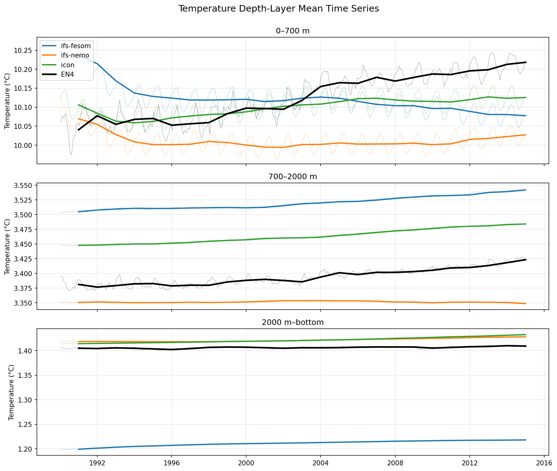
This figure displays volume-weighted mean ocean temperature time series for three depth layers (0-700 m, 700-2000 m, 2000 m-bottom) comparing three high-resolution models against EN4 observations from 1990 to roughly 2015.
Key Findings
- None of the models capture the strong upper-ocean (0-700 m) warming trend observed in EN4 over the simulated period.
- IFS-FESOM exhibits a strong initial cooling adjustment (drift) in the upper 700 m during the first 5-10 years, starting significantly warmer than observations.
- Significant mean-state biases exist in the intermediate (700-2000 m) and deep (2000 m-bottom) ocean: IFS-FESOM is too warm at intermediate depths and too cold in the deep ocean, while ICON is consistently too warm at intermediate depths.
Spatial Patterns
In the upper 700 m, observations show a clear warming trend (~0.15°C over 25 years), while models show either cooling (IFS-FESOM), flat evolution (IFS-NEMO), or weak warming (ICON). At 700-2000 m, observations show weak warming, while IFS-FESOM and ICON show stronger warming trends, indicating deep heat penetration or drift. In the deep ocean (>2000 m), temperatures are relatively stable across all datasets, though absolute mean states differ significantly.
Model Agreement
Model-observation agreement is poor regarding multi-decadal trends in the upper ocean. Inter-model spread is large in the mean state at all depths. For example, intermediate depth temperatures spread across ~0.15°C between IFS-NEMO (coldest) and IFS-FESOM (warmest), and deep ocean temperatures spread across ~0.2°C.
Physical Interpretation
The inability of the models to reproduce the observed 0-700 m warming trend suggests a deficiency in simulating the planetary energy imbalance or the efficiency of ocean heat uptake. The strong initial cooling in IFS-FESOM's upper ocean points to initialization shock, where the model adjusts rapidly to a state more consistent with its internal forcing and mixing physics. The steady warming of intermediate waters in IFS-FESOM and ICON may indicate excessive downward vertical mixing or spurious numerical diffusion of heat from the upper layers.
Caveats
- The 25-year simulation period makes it difficult to cleanly separate forced climate trends from model drift and internal multidecadal variability.
- Observational uncertainty in the EN4 dataset increases significantly below 700 m due to sparser sampling (especially prior to the full Argo deployment in the mid-2000s).
Temperature Hovmoller (first-timestep anomaly)
| Variables | avg_thetao, avg_so |
|---|---|
| Models | ifs-fesom, ifs-nemo, icon |
| Reference Dataset | EN4 v4.2.2 |
| Units | K |
| Period | 1990–2014 |
Summary high
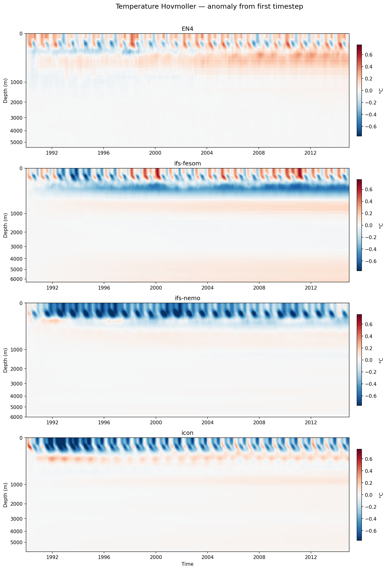
Time-depth Hovmoller diagrams of global-mean ocean temperature anomalies relative to the first timestep reveal significant and divergent intrinsic model drifts over the 1990–2014 period compared to the warming trend seen in EN4 observations.
Key Findings
- EN4 observations show a broad, progressive warming trend in the upper 1000m over the period, which is largely obscured in the models by intrinsic drifts.
- IFS-FESOM develops a severe, intensifying cold drift around 500m depth, accompanied by anomalous warming at ~1000m and in the abyssal ocean (>4000m).
- IFS-NEMO exhibits persistent cold anomalies concentrated in the upper 300m, while ICON contrasts with a distinct warm drift centered around 500m depth.
Spatial Patterns
The non-linear depth axis highlights upper-ocean changes. EN4 displays gradual decadal warming down to 1000m, becoming more prominent after 2000. In contrast, IFS-FESOM shows a stark, deepening cold anomaly band (exceeding -0.6°C) between 300m and 800m. IFS-NEMO's cold drift is shallower, dominating the upper 300m. ICON features a warm anomaly band (~0.4°C) around 500m. All models show strong surface anomalies reflecting the seasonal cycle relative to the initial month's state, but with varying amplitudes compared to EN4.
Model Agreement
There is poor agreement between the models and observations regarding long-term temperature trends, as model-specific initialization drifts dominate the anomalies. Inter-model agreement is also low; models diverge significantly on the sign and depth of subsurface drifts (e.g., FESOM cooling vs. ICON warming at 500m), though most share a faint warming tendency near 1000m.
Physical Interpretation
The prominent drifts indicate adjustment shocks and imbalances between the initial ocean state and each model's specific surface forcing (heat and momentum fluxes) and internal physics. FESOM's pronounced cooling at 500m suggests excessive subduction or vertical mixing of colder near-surface waters. ICON's mid-depth warming suggests contrasting biases, such as insufficient ventilation or excessive downward heat mixing. The shared warming at 1000m likely reflects a generalized adjustment of the global thermocline depth from its initialized state.
Caveats
- Calculating anomalies relative to a single first timestep aliases the seasonal cycle of that specific initial month into the long-term signal.
- The analysis conflates transient climate change (global warming) with intrinsic model drift (initialization shock), making it difficult to isolate the forced response.
Temperature Hovmoller (EN4-ref anomaly)
| Variables | avg_thetao, avg_so |
|---|---|
| Models | ifs-fesom, ifs-nemo, icon |
| Reference Dataset | EN4 v4.2.2 |
| Units | K |
| Period | 1990–2014 |
Summary high
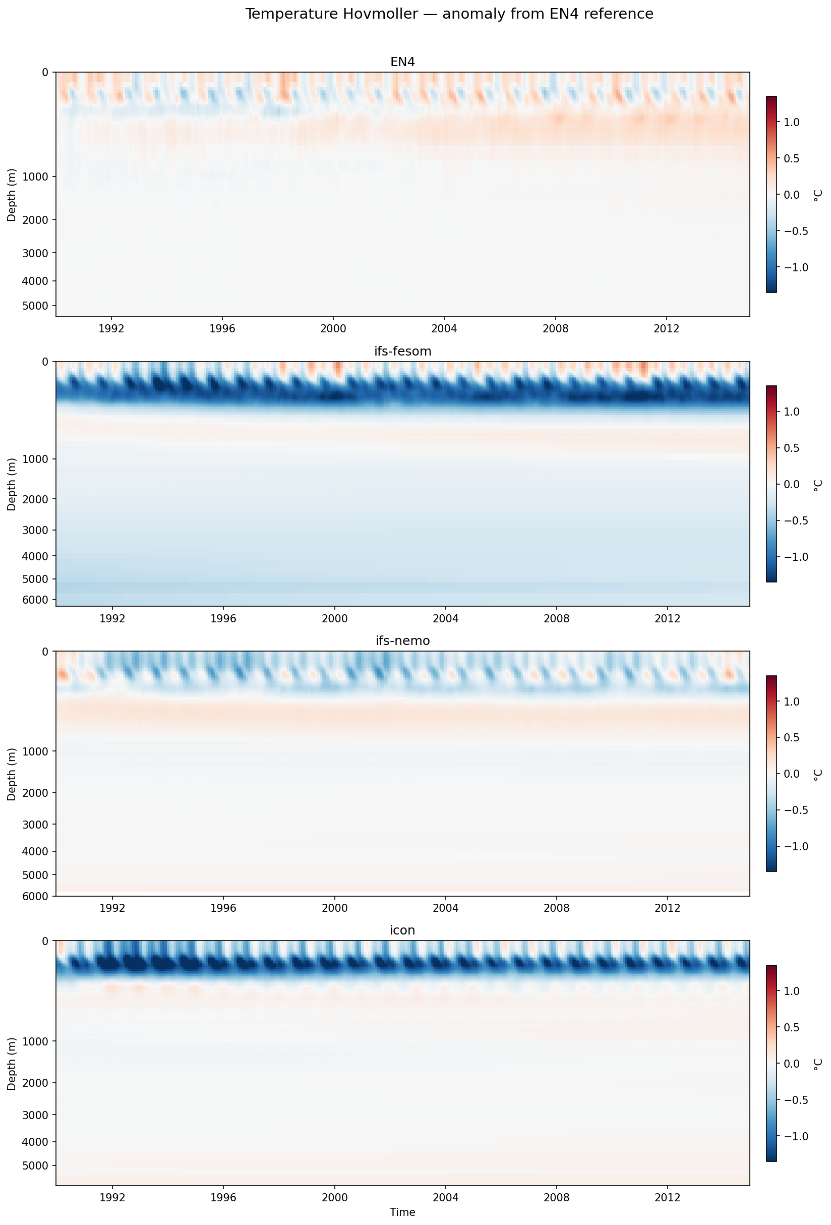
Time-depth Hovmoller diagrams display global-mean ocean temperature anomalies relative to the initial EN4 observational state from 1990-2014. The figure reveals striking upper-ocean cold biases in IFS-FESOM and ICON, contrasting with a more realistic multi-decadal evolution in IFS-NEMO.
Key Findings
- IFS-FESOM and ICON rapidly develop severe, persistent cold biases (exceeding -1.0 °C) in the upper 500 m.
- IFS-NEMO performs best among the models, better capturing the observed EN4 seasonal cycle and upper-ocean warming trend without massive mean-state drifts.
- Both IFS-FESOM and IFS-NEMO exhibit a persistent subsurface warm bias layer between roughly 500 m and 1000 m depth.
Spatial Patterns
EN4 observations show a clear multi-decadal warming trend in the upper 1000 m, with prominent seasonal cycles in the surface layer. In contrast, IFS-FESOM and ICON are dominated by a rapid initial adjustment that establishes long-lasting cold mean-state biases near the surface. The deep ocean (>2000 m) is relatively stable across all models, though IFS-FESOM exhibits a slight long-term cold drift near the bottom.
Model Agreement
Inter-model agreement is low in the upper ocean (0-500 m), where IFS-NEMO tracks observations reasonably well while IFS-FESOM and ICON diverge sharply with severe cold biases. The presence of a 500-1000 m warm bias in both IFS-coupled models (FESOM and NEMO) suggests a potential shared issue with the IFS atmospheric fluxes or wind stress, whereas ICON lacks this specific subsurface feature.
Physical Interpretation
The immediate onset of intense upper-ocean cold anomalies in IFS-FESOM and ICON points to a severe initialization shock, likely driven by an imbalance in net surface heat fluxes (excessive cooling) or overly vigorous vertical mixing drawing cold water upward. The subsurface warm anomalies (500-1000 m) seen in the IFS models may indicate overly shallow ventilation of intermediate water masses or spurious diapycnal mixing trapping heat at depth.
Caveats
- Global-mean profiles can mask severe, compensating regional biases (e.g., anomalous warming in one ocean basin offsetting extreme cooling in another).
- The analysis relies on the EN4 initial state as a strict baseline; uncertainties in early 1990s observational sampling (pre-Argo) may affect the interpretation of the reference profile.