Climate Variability (ERA5) — Feather — Climate Model Evaluation

Total Cloud Cover — Variability (STD)

Variables	clt
Models	ifs-fesom, ifs-nemo, CMIP6 MMM
Reference Dataset	ERA5
Units	%
Period	1990–2014
ifs-fesom	Std Gmean: 7.62 · Diff Gmean: 0.41 · Rmse: 1.14
ifs-nemo	Std Gmean: 7.60 · Diff Gmean: 0.38 · Rmse: 1.01
CMIP6 MMM	Std Gmean: 8.07 · Diff Gmean: 0.86 · Rmse: 1.33

Summary high

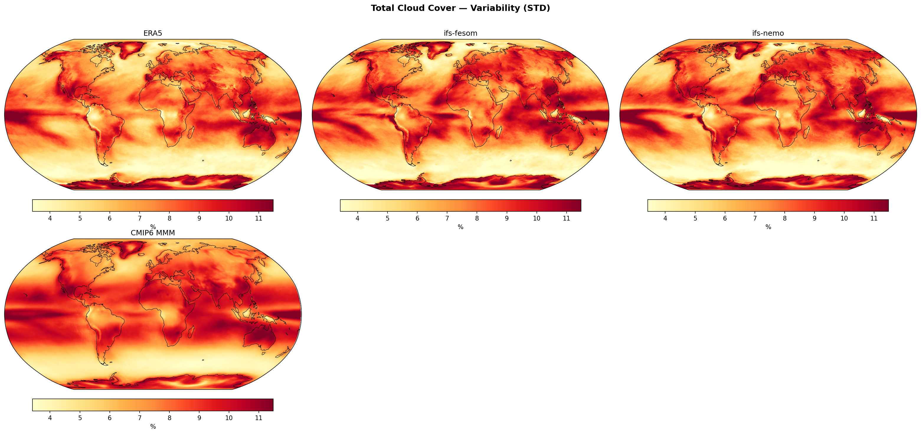
This figure illustrates the standard deviation of deseasonalised, detrended monthly Total Cloud Cover (TCC) for the period 1990–2014, comparing ERA5 reanalysis with IFS-FESOM, IFS-NEMO, and the CMIP6 multi-model mean.

Key Findings

Variability is highest (>10%) in the tropical convective zones (ITCZ, SPCZ, Maritime Continent) and the Southern Ocean storm track.
Both IFS models reproduce the spatial patterns of ERA5 with high fidelity, particularly the diagonal orientation of the SPCZ and the confinement of the ITCZ, improving upon the CMIP6 baseline.
IFS-NEMO shows slightly better agreement with observations (RMSE ~1.01%) compared to IFS-FESOM (RMSE ~1.14%), while the CMIP6 MMM significantly overestimates global variability (diff ~0.86%) and exhibits larger spatial errors.

Spatial Patterns

Dominant features include high variability bands in the tropical Pacific and Atlantic (associated with the ITCZ/SPCZ) and the mid-latitude storm tracks. Low variability (<5%) is found in the persistent stratocumulus regions off the western coasts of continents (e.g., Peru, Namibia, California) and over major desert regions like the Sahara and Australia. The tropical Pacific exhibits a distinct signature of interannual variability (likely ENSO-driven).

Model Agreement

The IFS models show excellent agreement with ERA5, capturing the magnitude and sharp gradients of variability in the tropics better than the CMIP6 MMM. The CMIP6 MMM displays a broader, more diffuse variability pattern and hints at a 'double ITCZ' bias in the Pacific (excessive zonal variability in the southern hemisphere tropics) which is largely corrected in the high-resolution IFS simulations.

Physical Interpretation

The variability in monthly cloud cover anomalies is primarily driven by interannual modes like ENSO (evident in the central/eastern Pacific) and variations in the location and intensity of the ITCZ and mid-latitude storm tracks. The high resolution of the DestinE models likely allows for a better representation of the sharp boundaries of these dynamical features compared to the coarser CMIP6 ensemble.

Caveats

The CMIP6 MMM panel likely represents the mean of the standard deviations of individual models; its smoothness is partly an artifact of averaging multiple models with slightly displaced features.
The analysis is based on monthly data, so synoptic-scale (daily) cloud variability is averaged out, leaving primarily intraseasonal to interannual signals.

Total Cloud Cover — Variability Bias (STD diff)

Variables	clt
Models	ifs-fesom, ifs-nemo, CMIP6 MMM
Reference Dataset	ERA5
Units	%
Period	1990–2014
ifs-fesom	Std Gmean: 7.62 · Diff Gmean: 0.41 · Rmse: 1.14
ifs-nemo	Std Gmean: 7.60 · Diff Gmean: 0.38 · Rmse: 1.01
CMIP6 MMM	Std Gmean: 8.07 · Diff Gmean: 0.86 · Rmse: 1.33

Summary high

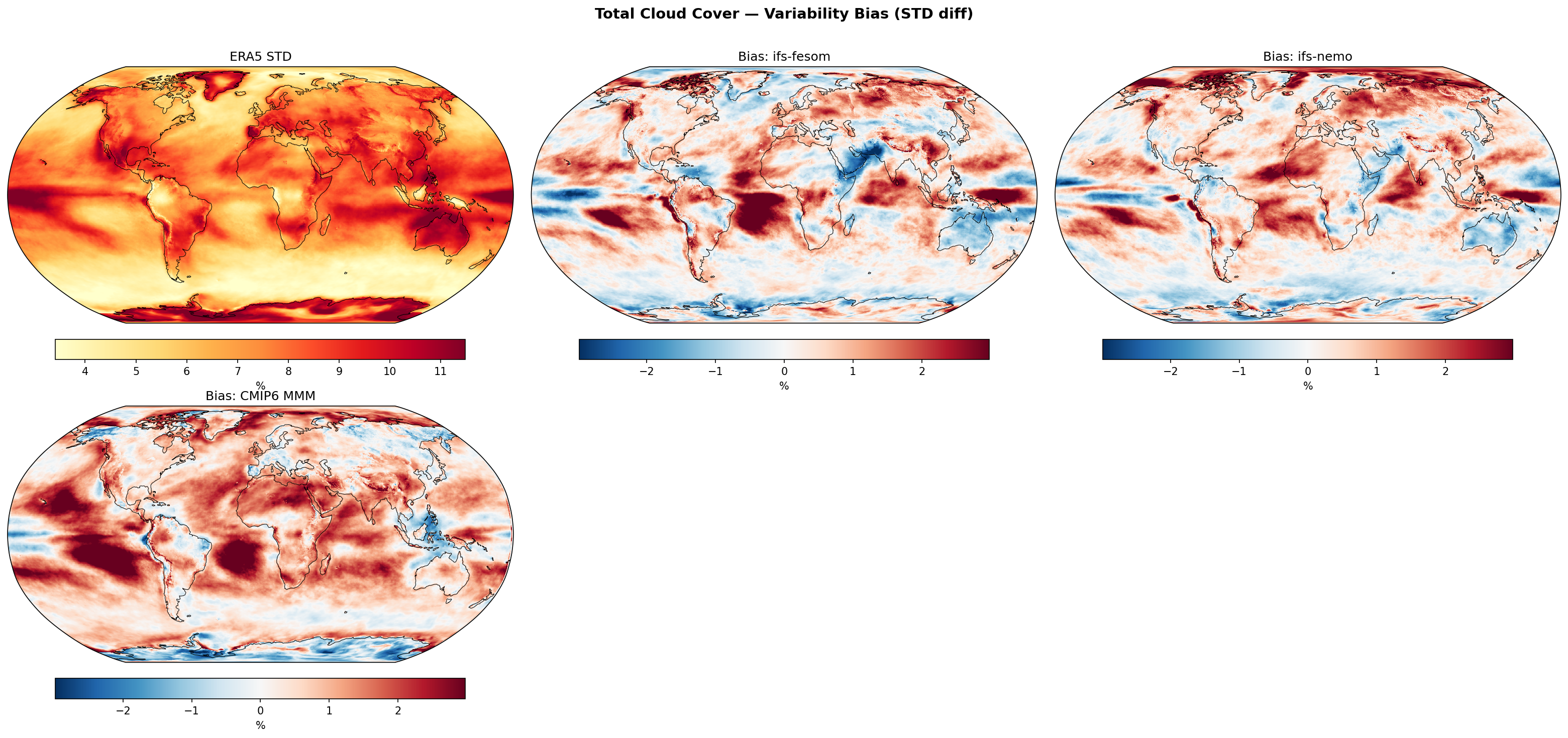
This diagnostic compares the temporal variability (standard deviation) of total cloud cover in high-resolution IFS-based simulations against ERA5 reanalysis and the CMIP6 multi-model mean. The IFS models (ifs-fesom and ifs-nemo) exhibit markedly better agreement with ERA5 than the CMIP6 ensemble, reducing global mean biases and RMSE significantly, though they share systematic regional biases in stratocumulus and convective zones.

Key Findings

IFS models outperform CMIP6 MMM, showing lower global mean bias (~0.4% vs 0.86%) and RMSE (~1.0-1.1% vs 1.33%).
A prominent bias dipole exists in the tropics: models overestimate variability in eastern boundary stratocumulus regions (e.g., off Peru, Namibia, California) and underestimate variability in the deep tropical convective zones (ITCZ/SPCZ).
ifs-fesom and ifs-nemo show nearly identical bias patterns, indicating that atmospheric physics (IFS) rather than the ocean coupling strategy dominates cloud variability errors.
CMIP6 MMM exhibits a widespread positive variability bias (overestimation) across most ocean basins and land masses, particularly severe in the Southern Ocean and subtropical stratocumulus decks.

Spatial Patterns

ERA5 shows peak variability (>10%) in the ITCZ and mid-latitude storm tracks. The IFS models capture the broad structure but systematically overestimate variability (red, >2% bias) in marine stratocumulus decks and the Arctic, while underestimating it (blue, <-2% bias) in the core of the tropical warm pool and ITCZ. The CMIP6 MMM shows a stronger and more spatially extensive positive bias, particularly over the Southern Hemisphere oceans and global land surfaces.

Model Agreement

There is exceptionally high agreement between ifs-fesom and ifs-nemo, suggesting the change in ocean model (unstructured FESOM vs structured NEMO) has negligible impact on cloud cover variability. Both IFS models diverge from the CMIP6 MMM, which is systematically 'noisier' (higher variability) relative to ERA5.

Physical Interpretation

The positive bias in eastern boundary upwelling regions suggests the models struggle to maintain persistent stratocumulus decks, likely oscillating between cloudy and clear states more frequently than the assimilated reanalysis. Conversely, the negative bias in the deep tropics implies that model convection is too persistent or stationary, lacking the temporal intermittency or propagation characteristics of observed weather systems (e.g., MJO modulation). The reduced bias in IFS compared to CMIP6 likely reflects the benefits of higher resolution in resolving synoptic-scale weather systems and cloud dynamics.

Caveats

ERA5 total cloud cover is a model-derived product constrained by observations, not a direct observation, and thus contains its own model biases.
The analysis period (1990-2014) captures the AMIP/historical overlap but does not account for potential non-stationarity in cloud trends.

Surface Latent Heat Flux — Variability (STD)

Variables	hfls
Models	ifs-fesom, ifs-nemo, icon
Reference Dataset	ERA5
Units	W/m2
Period	1990–2014
ifs-fesom	Std Gmean: 15.31 · Diff Gmean: 1.57 · Rmse: 3.84
ifs-nemo	Std Gmean: 14.99 · Diff Gmean: 1.24 · Rmse: 3.41
icon	Std Gmean: 13.65 · Diff Gmean: -0.09 · Rmse: 5.49

Summary high

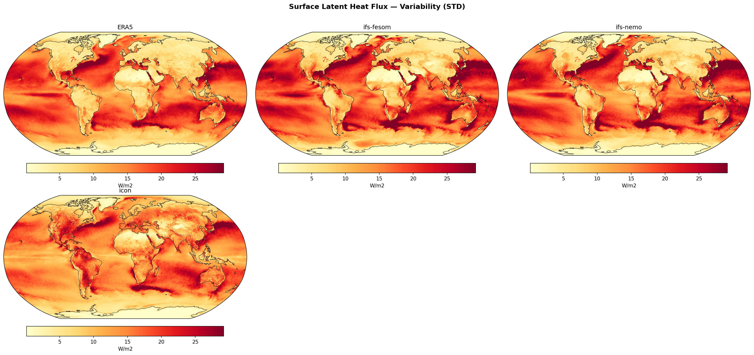
This diagnostic compares the interannual variability (standard deviation of monthly anomalies) of surface latent heat flux across three models and ERA5. The IFS-based models (ifs-fesom, ifs-nemo) closely reproduce observed oceanic patterns with slightly elevated amplitudes, while ICON exhibits distinct discrepancies, particularly excessive variability over land.

Key Findings

Western Boundary Currents (Gulf Stream, Kuroshio) and the Agulhas Return Current are correctly identified as regions of maximum variability (>25 W/m²) by all models.
IFS-nemo and ifs-fesom exhibit a systematic positive bias in variability amplitude (global mean excess of +1.24 and +1.57 W/m² respectively) but maintain high spatial correlation with ERA5.
ICON displays a distinct error pattern characterized by excessive, high-frequency spatial noise over continents (e.g., North America, Eurasia) and the highest RMSE (5.49 W/m²), despite having a near-zero global mean bias.

Spatial Patterns

The dominant spatial feature in ERA5 is the contrast between high variability in Western Boundary Currents and the tropical Pacific (ENSO signature) versus lower variability in the stable subtropical gyres. Over land, variability is generally lower than over the oceans in ERA5. The IFS models amplify these oceanic patterns, particularly in the Southern Ocean. In contrast, ICON shows a 'granular' texture with unrealistically high variability scattered across continental landmasses.

Model Agreement

The two IFS-based models show strong mutual agreement and good structural agreement with ERA5, with ifs-nemo performing slightly better (lower RMSE) than ifs-fesom. ICON is an outlier, diverging significantly in its land-surface representation.

Physical Interpretation

Oceanic variability is driven by SST anomalies (e.g., ENSO) and strong air-sea interaction in eddy-rich regions (WBCs). The IFS models' slight overestimation suggests energetic coupling or intense surface wind variability. ICON's excessive land variability implies issues with the land-surface scheme (e.g., soil moisture memory) or precipitation forcing, causing surface fluxes to react too strongly to atmospheric forcing.

Caveats

The analysis uses monthly means, smoothing out synoptic-scale variability.
The 'noise' in ICON over land might be related to grid-point storms or specific land-surface parameterization instabilities.

Surface Latent Heat Flux — Variability Bias (STD diff)

Variables	hfls
Models	ifs-fesom, ifs-nemo, icon
Reference Dataset	ERA5
Units	W/m2
Period	1990–2014
ifs-fesom	Std Gmean: 15.31 · Diff Gmean: 1.57 · Rmse: 3.84
ifs-nemo	Std Gmean: 14.99 · Diff Gmean: 1.24 · Rmse: 3.41
icon	Std Gmean: 13.65 · Diff Gmean: -0.09 · Rmse: 5.49

Summary high

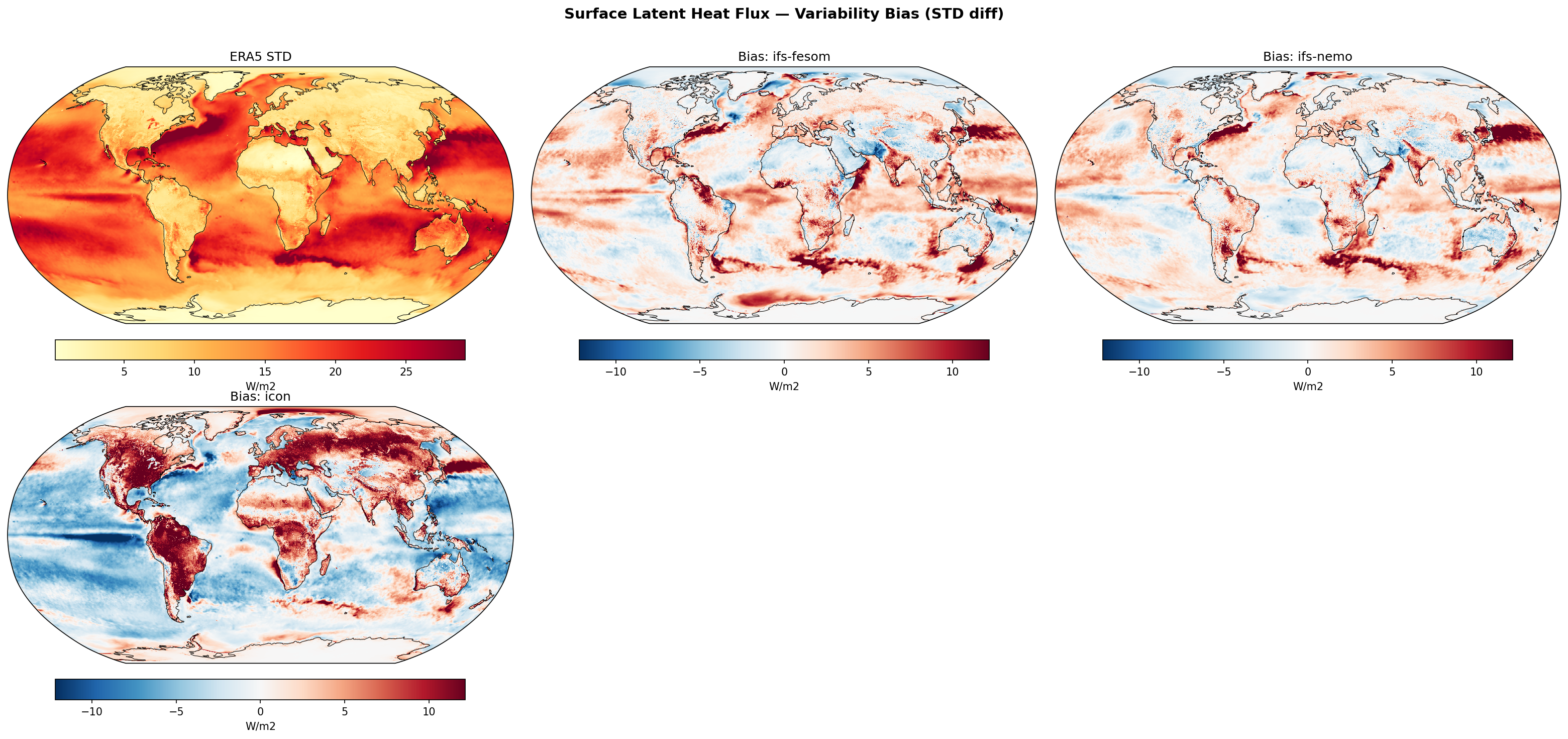
This figure evaluates the interannual variability of surface latent heat flux (SLHF) by comparing the standard deviation of model output against ERA5. IFS-based models generally exhibit higher variability than ERA5, particularly in energetic ocean regions, whereas ICON displays a distinct dichotomy of suppressed ocean variability and excessive land variability.

Key Findings

IFS-FESOM and IFS-NEMO show strong positive variability biases in Western Boundary Currents (Gulf Stream, Kuroshio) and the Agulhas region, indicating more energetic air-sea interaction than ERA5.
ICON exhibits a stark land-ocean contrast: widespread negative variability bias over the global oceans (too stable) but severe positive bias over land, particularly in boreal and tropical forests.
All models overestimate SLHF variability over tropical rainforests (Amazon, Congo, Maritime Continent), with ICON showing the largest errors (>10 W/m²).
IFS-FESOM and IFS-NEMO share very similar bias patterns, confirming that the atmospheric component (IFS) dominates the surface flux variability characteristics.

Spatial Patterns

ERA5 shows peak variability in Western Boundary Currents and trade wind belts. IFS models exaggerate this pattern, with red patches (positive bias) aligned with the Gulf Stream, Kuroshio, and Southern Ocean sea-ice edge. They also show negative biases in the eastern tropical Pacific and North Atlantic subpolar gyre. ICON deviates significantly, with blue (negative bias) dominating the oceans and dark red (positive bias) covering high-latitude and tropical landmasses.

Model Agreement

High agreement between IFS-FESOM and IFS-NEMO (RMSE ~3.4-3.8 W/m²), reflecting their shared atmospheric model. ICON is an outlier (RMSE ~5.5 W/m²), disagreeing with the IFS models in sign over most of the ocean and magnitude over land.

Physical Interpretation

The positive bias in Western Boundary Currents for IFS models likely results from high resolution (~5-10 km) resolving sharper SST fronts and mesoscale eddies than the coarser ERA5 (~31 km), leading to stronger turbulent heat flux variability. The severe positive land bias in ICON suggests overly sensitive soil moisture-evaporation feedbacks or issues in the land-surface parameterisation (JSBACH). The suppressed ocean variability in ICON may indicate weaker surface wind variability or dampened air-sea coupling in the tropics.

Caveats

ERA5 fluxes are derived from bulk formulae and assimilation rather than direct observation; errors in ERA5's boundary layer or SSTs could influence the reference baseline.
The 'variability' metric (STD) combines intrinsic variability and potential model drift if not perfectly detrended, though the pattern suggests interannual physical variability.

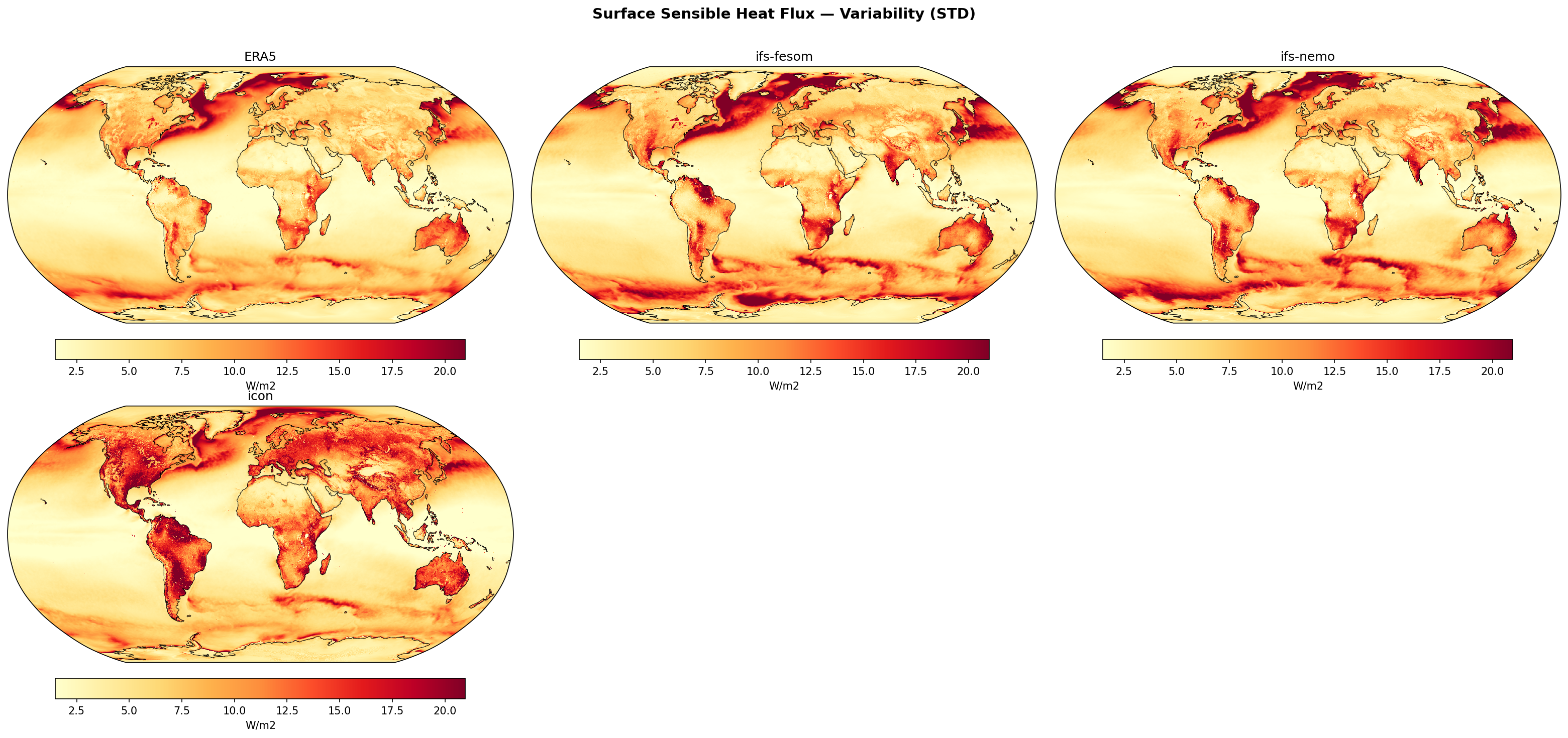
Surface Sensible Heat Flux — Variability (STD)

Variables	hfss
Models	ifs-fesom, ifs-nemo, icon
Reference Dataset	ERA5
Units	W/m2
Period	1990–2014
ifs-fesom	Std Gmean: 6.76 · Diff Gmean: 0.87 · Rmse: 2.80
ifs-nemo	Std Gmean: 6.64 · Diff Gmean: 0.74 · Rmse: 2.36
icon	Std Gmean: 7.06 · Diff Gmean: 1.17 · Rmse: 4.14

Summary high

This figure compares the temporal variability (standard deviation of deseasonalised anomalies) of surface sensible heat flux (SSHF) across three high-resolution coupled models against ERA5 reanalysis for the period 1990–2014. It highlights regions of strong turbulent heat exchange over Western Boundary Currents and continental surfaces.

Key Findings

All models successfully reproduce the observation-based spatial maxima in SSHF variability (>17.5 W/m²) associated with major ocean currents (Gulf Stream, Kuroshio, Agulhas) and the North Atlantic storm track.
ifs-nemo demonstrates the highest fidelity to ERA5, with the lowest global RMSE (2.36 W/m²) and very similar spatial structures over both land and ocean.
ICON exhibits a systematic overestimation of SSHF variability over global land masses (particularly in boreal Eurasia/North America and tropical basins like the Amazon), resulting in a significantly higher RMSE (4.14 W/m²) compared to the IFS-based models.

Spatial Patterns

In ERA5, oceanic variability peaks in Western Boundary Currents and high-latitude storm tracks, driven by air-sea interaction. Over land, variability is highest in semi-arid/transition regions (e.g., Australia, Western US, Sahel) where soil moisture limitations modulate the Bowen ratio. The marginal sea ice zones also show elevated variability due to the fluctuating presence of insulating ice versus open water.

Model Agreement

ifs-fesom and ifs-nemo show strong inter-model agreement and close alignment with ERA5 (RMSE ~2.4–2.8 W/m²). ICON agrees well with ERA5 over the oceans but diverges significantly over land, displaying widespread excessive variability (dark red regions) in areas where ERA5 shows moderate or low variability.

Physical Interpretation

Oceanic variability is driven by synoptic atmospheric events (e.g., cold air outbreaks) passing over sharp SST gradients in eddy-rich regions. The excessive land variability in ICON suggests potential sensitivities in its land surface coupling (possibly related to soil moisture memory, surface roughness, or aerodynamic resistance schemes) that allow surface temperature and fluxes to fluctuate more rapidly than in ERA5 or IFS models.

Caveats

ERA5 surface fluxes are derived from model physics constrained by atmospheric observations, not direct measurements, so they act as a model-consistent reference rather than ground truth.
The cause of ICON's excessive land variability cannot be fully diagnosed without inspecting latent heat flux and soil moisture variability.

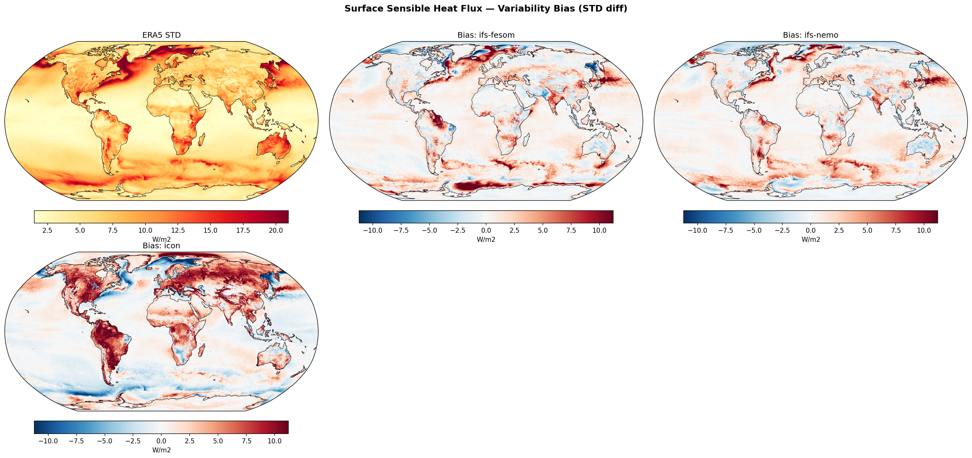
Surface Sensible Heat Flux — Variability Bias (STD diff)

Variables	hfss
Models	ifs-fesom, ifs-nemo, icon
Reference Dataset	ERA5
Units	W/m2
Period	1990–2014
ifs-fesom	Std Gmean: 6.76 · Diff Gmean: 0.87 · Rmse: 2.80
ifs-nemo	Std Gmean: 6.64 · Diff Gmean: 0.74 · Rmse: 2.36
icon	Std Gmean: 7.06 · Diff Gmean: 1.17 · Rmse: 4.14

Summary high

This figure evaluates the variability (standard deviation) of Surface Sensible Heat Flux (SSHF) in three high-resolution models against ERA5 reanalysis. While ocean variability patterns broadly align with observations (peaking in Western Boundary Currents), there are significant divergences over land, most notably a severe, global overestimation of variability in the ICON model.

Key Findings

ICON exhibits a drastic positive bias in SSHF variability over nearly all land masses, with excesses often exceeding 10 W/m², leading to the highest RMSE (4.14 W/m²).
Both IFS-based models (ifs-fesom and ifs-nemo) overestimate variability over tropical continents (Amazon, Central Africa) and Western Boundary Currents (Gulf Stream, Kuroshio), but are generally closer to ERA5 than ICON.
IFS-NEMO performs best statistically (RMSE 2.36 W/m²), slightly outperforming IFS-FESOM (RMSE 2.80 W/m²), particularly in the high-latitude oceans.
Models tend to underestimate variability (negative bias) in the sea-ice marginal zones of the Southern Ocean and parts of the subpolar North Atlantic.

Spatial Patterns

ERA5 shows peak variability in Western Boundary Currents and arid continental regions. The IFS models replicate the ocean peaks but exaggerate their magnitude and extent, while also showing localized high variability over tropical rainforests. ICON's spatial pattern is dominated by a stark land-sea contrast: intense positive bias over almost all continents and mild negative bias (underestimation of variability) over tropical and subtropical oceans.

Model Agreement

The two IFS models show strong agreement in their land biases (likely due to the shared atmospheric component) and similar structures in the North Atlantic, though IFS-FESOM has stronger biases in the Labrador Sea. ICON is an outlier with distinct and much larger errors over land.

Physical Interpretation

The extreme land variability in ICON suggests issues with its land surface model (TERRA) or land-atmosphere coupling, possibly related to overly responsive surface temperatures or soil moisture partitioning that fluctuates too widely on synoptic timescales. The positive ocean biases in the Gulf Stream and Kuroshio for IFS models are typical of high-resolution simulations where sharp SST gradients induce energetic air-sea interaction (cold air outbreaks) that may exceed the smoothed variability found in ERA5. The tropical land biases in IFS may relate to convective triggering and associated surface flux variability.

Caveats

ERA5 fluxes are model-derived products (constrained by assimilation) rather than direct observations, so biases may partly reflect differences in bulk formula parameterizations.
The analysis does not distinguish between synoptic (weather) variability and seasonal cycle amplitude contributions to the total standard deviation.

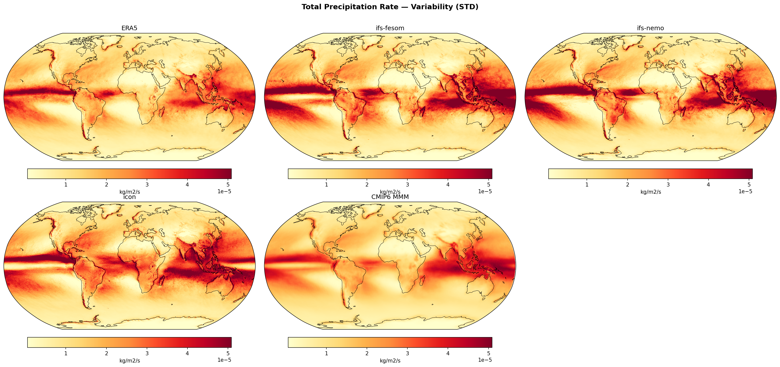
Total Precipitation Rate — Variability (STD)

Variables	pr
Models	ifs-fesom, ifs-nemo, icon, CMIP6 MMM
Reference Dataset	ERA5
Units	kg/m2/s
Period	1990–2014
ifs-fesom	Std Gmean: 0.00 · Diff Gmean: 0.00 · Rmse: 0.00
ifs-nemo	Std Gmean: 0.00 · Diff Gmean: 0.00 · Rmse: 0.00
icon	Std Gmean: 0.00 · Diff Gmean: 0.00 · Rmse: 0.00
CMIP6 MMM	Std Gmean: 0.00 · Diff Gmean: 0.00 · Rmse: 0.00

Summary high

This diagnostic compares the interannual variability (standard deviation of deseasonalised, detrended monthly anomalies) of total precipitation rates across three high-resolution DestinE models (ifs-fesom, ifs-nemo, icon) and the CMIP6 multi-model mean against ERA5 reanalysis.

Key Findings

All three high-resolution models overestimate precipitation variability compared to ERA5, with positive global mean bias differences ranging from ~2.9e-6 to 4.2e-6 kg/m²/s.
IFS-NEMO exhibits the best performance among the high-resolution models, having the lowest RMSE (8.19e-6 kg/m²/s) and smallest mean bias relative to ERA5.
ICON shows the strongest overestimation of variability, particularly in the tropical Pacific and Indian Ocean, with the highest RMSE (9.72e-6 kg/m²/s).
The CMIP6 Multi-Model Mean (MMM) shows the lowest variability and best statistical agreement with ERA5 (RMSE 4.97e-6 kg/m²/s), though its spatial pattern is notably smoother and less structurally resolved than the high-resolution simulations.

Spatial Patterns

Variability is dominated by the tropical convergence zones (ITCZ, SPCZ) and the Indian Monsoon region. The high-resolution models display very sharp, intense bands of variability in the ITCZ and SPCZ, often extending further east in the Pacific than observed in ERA5 (suggestive of a double-ITCZ bias signature). Orographic precipitation variability (Andes, Himalayas) is keenly resolved in the DestinE models compared to the diffuse CMIP6 patterns. The Maritime Continent shows particularly intense variability in the models compared to ERA5.

Model Agreement

The DestinE models (ifs-fesom, ifs-nemo, icon) agree on the spatial structure of excess variability in the tropics, all showing 'hotter' variability than ERA5. IFS-FESOM and IFS-NEMO are spatially very similar, confirming that the ocean coupling method (unstructured FESOM vs structured NEMO) has a secondary effect on atmospheric precip variability compared to the atmospheric model formulation. ICON diverges slightly with the highest intensity of variability.

Physical Interpretation

The high precipitation variability in the tropics is driven by ENSO dynamics and convective activity. The high-resolution models likely produce more intense convective events and possibly stronger ENSO amplitude or tropical instability waves than the reanalysis or the smoothed CMIP6 ensemble. The explicit resolving of smaller-scale vertical velocities in high-resolution runs contributes to higher variance (grid-scale storms) compared to lower-resolution parameterized convection.

Caveats

Precipitation in ERA5 is a forecast product (generated by the model physics) rather than a direct assimilation, so it contains its own biases.
The CMIP6 MMM likely represents the mean of the standard deviations, which spatially smooths the field, naturally reducing localized extremes compared to single realizations of high-res models.

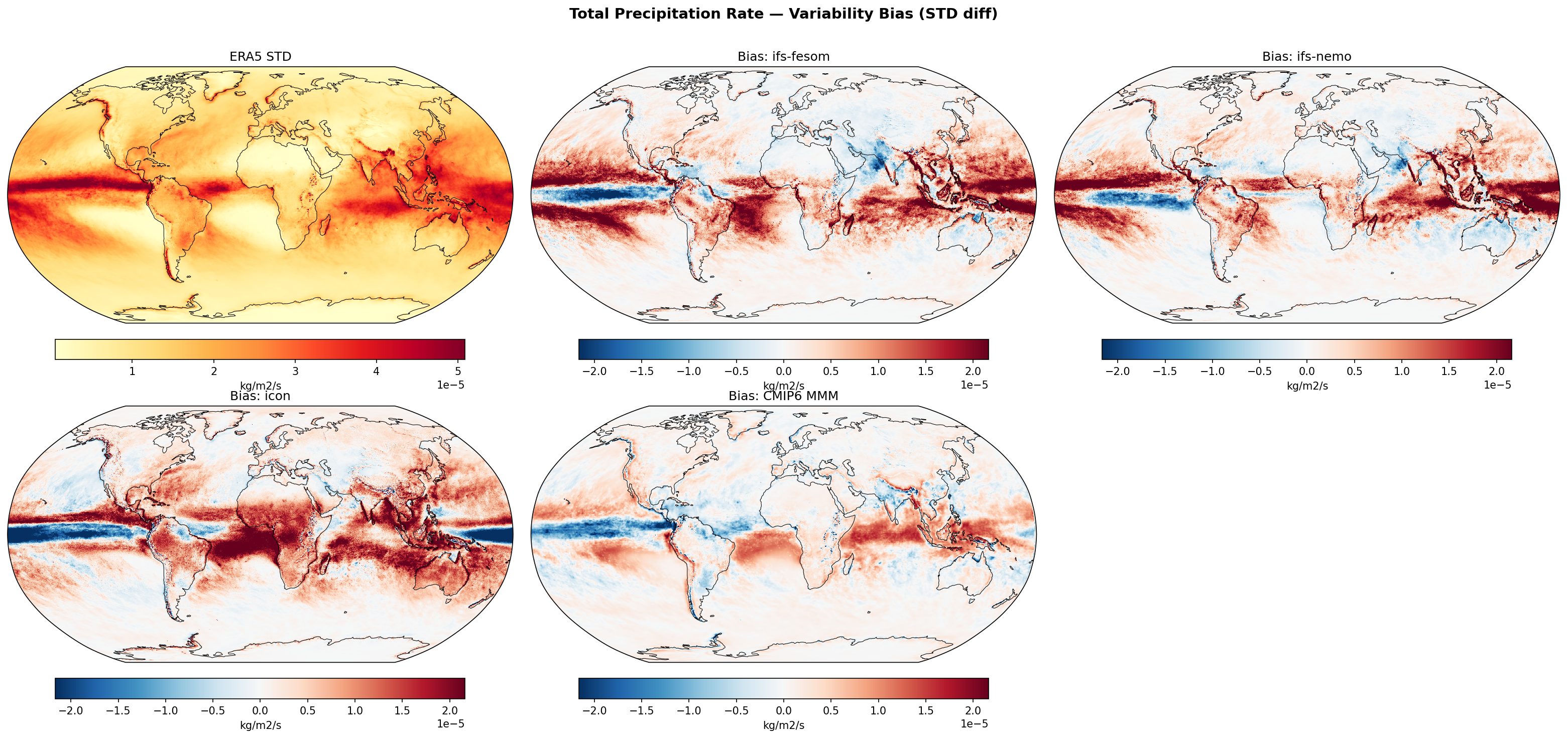
Total Precipitation Rate — Variability Bias (STD diff)

Variables	pr
Models	ifs-fesom, ifs-nemo, icon, CMIP6 MMM
Reference Dataset	ERA5
Units	kg/m2/s
Period	1990–2014
ifs-fesom	Std Gmean: 0.00 · Diff Gmean: 0.00 · Rmse: 0.00
ifs-nemo	Std Gmean: 0.00 · Diff Gmean: 0.00 · Rmse: 0.00
icon	Std Gmean: 0.00 · Diff Gmean: 0.00 · Rmse: 0.00
CMIP6 MMM	Std Gmean: 0.00 · Diff Gmean: 0.00 · Rmse: 0.00

Summary high

This diagnostic compares the standard deviation of monthly total precipitation rate in high-resolution DestinE models and the CMIP6 multi-model mean against ERA5 reanalysis. The models generally overestimate precipitation variability in the tropical off-equatorial regions and over land, while systematically underestimating variability along the equatorial Pacific.

Key Findings

All models exhibit a distinct zonal band of negative variability bias (blue) along the equatorial Pacific, indicating suppressed convective variance likely linked to cold tongue SST biases.
ICON shows the largest positive biases (excess variability) over the tropical oceans and continents, particularly the Amazon, Central Africa, and the Maritime Continent, resulting in the highest RMSE.
IFS-FESOM and IFS-NEMO share very similar bias patterns, with strong positive variability biases in the SPCZ and Indian Ocean, though IFS-NEMO performs slightly better (lower RMSE) than FESOM.
The CMIP6 MMM displays the lowest RMSE and smoothest fields but shares the systematic 'double ITCZ' variability structure (blue equator, red flanks) seen in the high-resolution simulations.

Spatial Patterns

The dominant pattern is a dipole in the tropical Pacific: suppressed variability along the equator flanked by bands of excess variability in the ITCZ and SPCZ regions. Over the Indian Ocean and tropical land masses (South America, Africa), the models (especially ICON) show widespread positive variability biases. Extratropical storm tracks show relatively smaller biases compared to the tropics.

Model Agreement

There is strong inter-model agreement on the spatial structure of biases, particularly the Pacific dipole and Indian Ocean excess. However, they diverge in magnitude: ICON produces significantly higher variability amplitudes than the IFS variants. The IFS-NEMO and IFS-FESOM patterns are nearly identical, indicating atmospheric physics dominates the signal over the specific ocean model used.

Physical Interpretation

The negative bias along the Pacific equator suggests models lock the ITCZ too firmly off-equator or have a cold SST bias that suppresses the deep convection associated with ENSO variability. The positive bias bands flanking the equator are consistent with the 'double ITCZ' syndrome, where models produce too much precipitation (and thus variability) in the southern branch. The excess variability over land in ICON may point to an overly responsive convective parameterization.

Caveats

The CMIP6 MMM likely represents the mean of individual model STDs; if it were the STD of the MMM, values would be artificially low.
Precipitation variability is strongly coupled to mean state biases; regions with excessive mean precipitation often show excessive variability.

Mean Sea Level Pressure — Variability (STD)

Variables	psl
Models	ifs-fesom, ifs-nemo, icon, CMIP6 MMM
Reference Dataset	ERA5
Units	Pa
Period	1990–2014
ifs-fesom	Std Gmean: 234.58 · Diff Gmean: 2.54 · Rmse: 23.32
ifs-nemo	Std Gmean: 237.60 · Diff Gmean: 5.55 · Rmse: 25.09
icon	Std Gmean: 227.90 · Diff Gmean: -4.14 · Rmse: 28.93
CMIP6 MMM	Std Gmean: 247.65 · Diff Gmean: 15.68 · Rmse: 27.54

Summary high

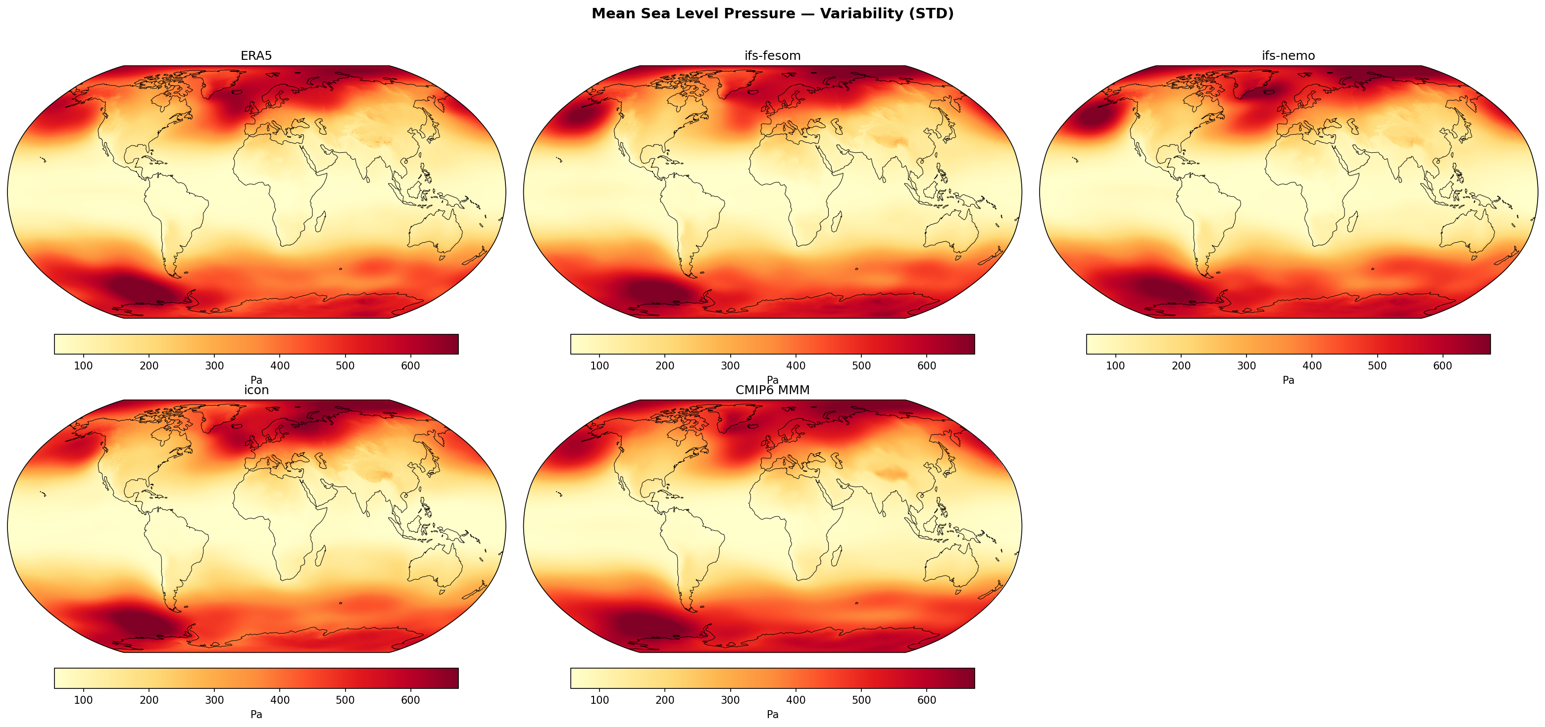
The figure illustrates the standard deviation of deseasonalised MSLP, acting as a proxy for storm track activity and internal variability. All high-resolution DestinE models (IFS-FESOM, IFS-NEMO, ICON) excellent capture the spatial structure of global pressure variability, with IFS-FESOM providing the closest statistical match to ERA5.

Key Findings

High MSLP variability (>600 Pa) is correctly located in the North Atlantic (Icelandic Low), North Pacific (Aleutian Low), and the Southern Ocean storm track belt.
IFS-FESOM exhibits the lowest global RMSE (23.3 Pa) and a small positive bias (+2.5 Pa), showing remarkable agreement with ERA5.
ICON slightly underestimates variability (global mean difference -4.1 Pa), visibly showing reduced intensity in the North Atlantic and North Pacific storm track centers compared to ERA5.
CMIP6 MMM overestimates global mean variability (+15.7 Pa) and displays smoother spatial gradients typical of ensemble averaging, contrasting with the sharper features of the high-resolution models.

Spatial Patterns

Dominant features include zonal bands of high variability in the Southern Hemisphere (40-65°S) and distinct localized maxima in the Northern Hemisphere extratropics corresponding to the termini of storm tracks. The tropics consistently show low variability (<200 Pa).

Model Agreement

There is high inter-model consistency regarding the location of variability centers. IFS-FESOM and IFS-NEMO align closely with ERA5 in magnitude. ICON is the only model to show a negative global bias, implying slightly damped synoptic activity. The CMIP6 ensemble mean is notably more variable globally than the high-resolution single realisations.

Physical Interpretation

MSLP variability primarily reflects synoptic-scale cyclone activity (storm tracks) and low-frequency variability modes (e.g., NAO, SAM, PNA). The maxima in the North Atlantic and Pacific correspond to regions where extratropical cyclones frequently deepen and stall. The tropical minimum reflects the weak pressure gradients and geostrophic balance regimes of the Hadley circulation.

Caveats

The CMIP6 MMM represents an average of multiple models, which inherently smoothes spatial noise but robustly identifies systematic signal; its high bias suggests many CMIP6 models may be too active.
Analysis uses deseasonalised data, so it specifically characterizes inter-monthly and inter-annual internal variability rather than the seasonal cycle amplitude.

Mean Sea Level Pressure — Variability Bias (STD diff)

Variables	psl
Models	ifs-fesom, ifs-nemo, icon, CMIP6 MMM
Reference Dataset	ERA5
Units	Pa
Period	1990–2014
ifs-fesom	Std Gmean: 234.58 · Diff Gmean: 2.54 · Rmse: 23.32
ifs-nemo	Std Gmean: 237.60 · Diff Gmean: 5.55 · Rmse: 25.09
icon	Std Gmean: 227.90 · Diff Gmean: -4.14 · Rmse: 28.93
CMIP6 MMM	Std Gmean: 247.65 · Diff Gmean: 15.68 · Rmse: 27.54

Summary high

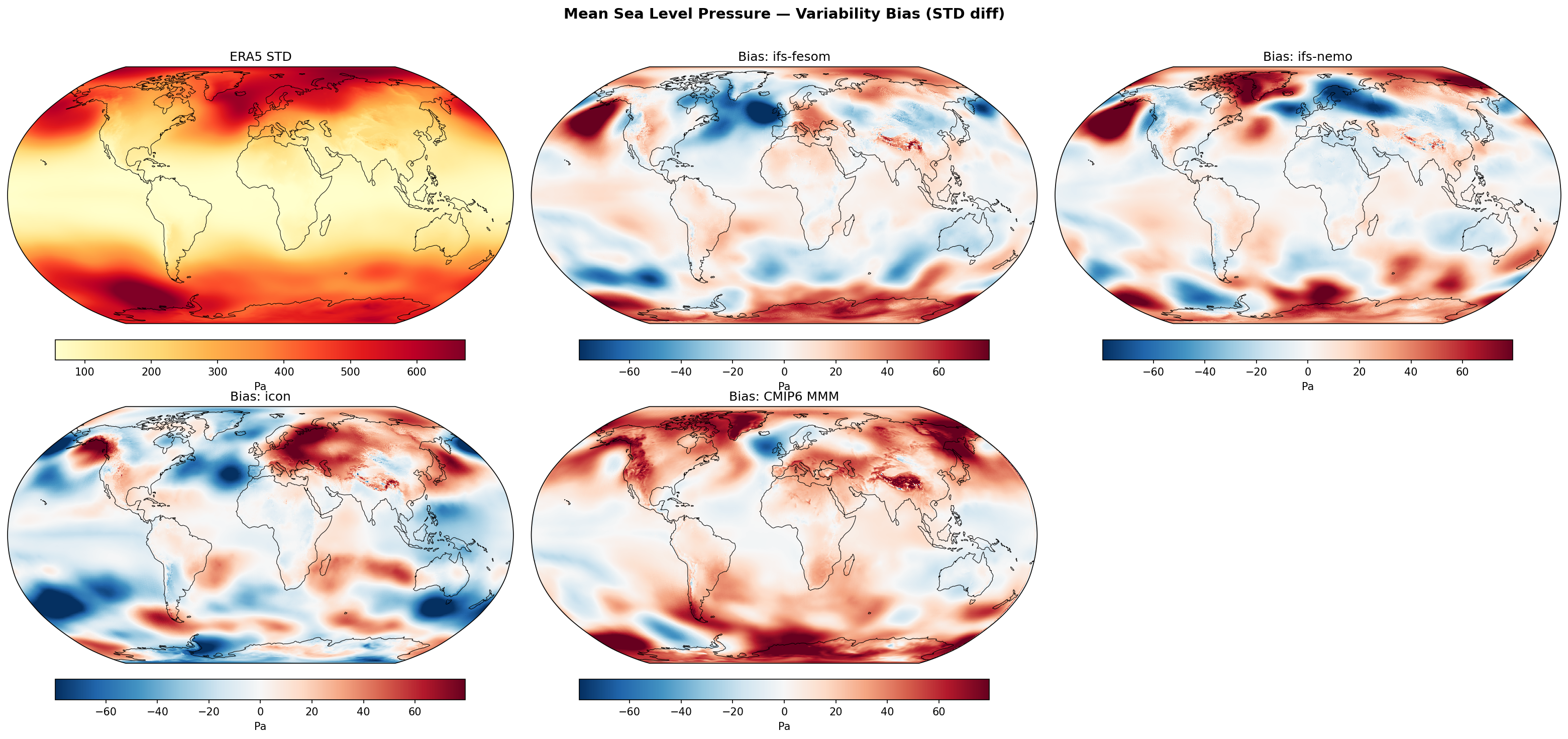
This diagnostic compares the variability (standard deviation) of Mean Sea Level Pressure (MSLP) in ERA5 against three high-resolution DestinE models and the CMIP6 multi-model mean, highlighting that the high-resolution simulations generally reduce the systematic positive variability bias found in CMIP6.

Key Findings

ifs-fesom achieves the lowest global RMSE (23.3 Pa) and smallest mean bias (+2.5 Pa), though it tends to underestimate variability in the core North Atlantic and North Pacific storm tracks.
icon displays a distinct land-sea bias contrast, with strong underestimation of variability over the central North Pacific and Atlantic oceans, but significant overestimation (red) over high-latitude land areas like Scandinavia and Northern Russia.
ifs-nemo exhibits generally higher variability than ifs-fesom, leading to positive biases in the Southern Ocean and parts of the North Atlantic, suggesting that the ocean model coupling (NEMO vs FESOM) strongly influences high-latitude atmospheric variance.
The CMIP6 MMM shows a systematic global overestimation of MSLP variability (mean bias +15.7 Pa), particularly intense in the Southern Ocean and Northern Hemisphere storm tracks, which the high-resolution models largely correct or over-correct.

Spatial Patterns

ERA5 shows peak MSLP variability (>500 Pa) in the major storm tracks (Aleutian Low, Icelandic Low, Southern Ocean). While CMIP6 exaggerates this variability everywhere, ifs-fesom and icon exhibit 'blue' negative bias patches in the center of the North Pacific and Atlantic storm tracks. icon uniquely shows strong 'red' positive biases over Northern Eurasia.

Model Agreement

The models diverge significantly in the extratropics. ifs-fesom and icon agree on underestimating North Pacific variability, whereas ifs-nemo is closer to neutral there. In the Southern Ocean, ifs-nemo aligns more with CMIP6 (positive bias) while icon is negatively biased. ifs-fesom and ifs-nemo differ notably despite sharing the IFS atmosphere, highlighting the role of air-sea coupling.

Physical Interpretation

MSLP variability on these timescales proxies for storm track activity and low-frequency modes (e.g., blocking, NAO/SAM). The underestimation in ifs-fesom and icon over oceans suggests reduced storm track intensity or persistence compared to ERA5. The strong positive bias in icon over Scandinavia implies excessive blocking frequency or intensity in that sector. The general reduction of the CMIP6 positive bias by high-res models suggests that increased resolution may improve the representation of energy dissipation or the lifetime of synoptic eddies.

Caveats

Units are in Pascals (Pa), so a bias of 60 Pa corresponds to 0.6 hPa, which is relatively small compared to the total variance but spatially coherent.
The analysis refers to monthly variability (based on standard diagnostic configurations), so it captures low-frequency dynamics rather than daily storminess.

Surface Downwelling Longwave — Variability (STD)

Variables	rlds
Models	ifs-fesom, ifs-nemo, icon, CMIP6 MMM
Reference Dataset	ERA5
Units	W/m2
Period	1990–2014
ifs-fesom	Std Gmean: 7.65 · Diff Gmean: 0.60 · Rmse: 1.32
ifs-nemo	Std Gmean: 7.47 · Diff Gmean: 0.42 · Rmse: 1.10
icon	Std Gmean: 7.10 · Diff Gmean: 0.05 · Rmse: 1.55
CMIP6 MMM	Std Gmean: 8.02 · Diff Gmean: 0.98 · Rmse: 1.35

Summary high

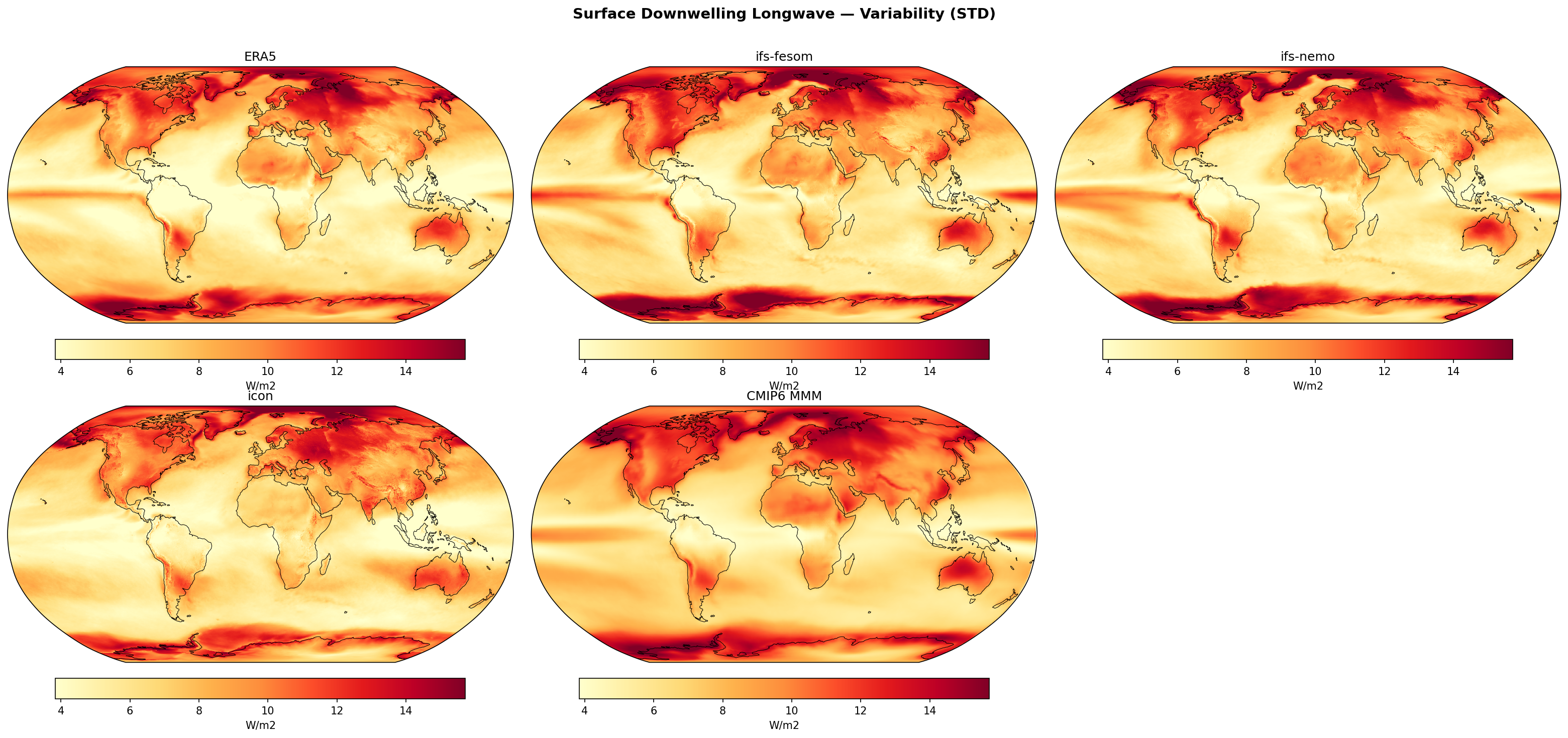
This diagnostic evaluates the variability (standard deviation) of deseasonalised surface downwelling longwave radiation (rlds), highlighting how models capture fluctuations driven by atmospheric temperature and cloud cover. While all high-resolution models reproduce the dominant land-sea contrast and tropical convective bands better than the CMIP6 baseline, IFS-NEMO shows the best overall agreement with ERA5, whereas ICON exhibits distinct regional biases over Southern Hemisphere landmasses.

Key Findings

Spatial maxima are correctly located over Northern Hemisphere high-latitude continents (>14 W/m²) and tropical convective zones (ITCZ/SPCZ), reflecting strong synoptic temperature variance and intermittent cloud forcing respectively.
IFS-NEMO demonstrates the highest skill (lowest RMSE of 1.10 W/m²) and realistic spatial patterns, followed closely by IFS-FESOM (RMSE 1.32 W/m²); both have a moderate positive global bias (~0.4-0.6 W/m²).
ICON displays the lowest global mean bias (+0.05 W/m²) but the highest spatial error (RMSE 1.55 W/m²), driven by excessive variability over semi-arid Southern Hemisphere land regions (Australia, South Africa, South America) and suppressed variability in the Weddell Sea.
The CMIP6 Multi-Model Mean systematically overestimates global variability (bias +0.98 W/m²) and exhibits smoothed gradients, particularly broadening the tropical convective bands compared to the sharper structures in ERA5 and high-resolution models.

Spatial Patterns

Variability is inherently higher over land due to lower heat capacity allowing larger temperature swings, particularly in NH winter regions (Siberia/Canada). Distinct bands of variability trace the ITCZ and SPCZ over the oceans. ICON specifically exaggerates variability over SH arid regions (e.g., Australia) relative to ERA5.

Model Agreement

IFS-NEMO shows the best agreement with ERA5. IFS-FESOM is very similar but slightly more energetic (higher bias). ICON diverges significantly over SH land, suggesting a specific issue with land-surface coupling or clear-sky radiative processes in those regimes.

Physical Interpretation

Longwave variability is primarily driven by near-surface air temperature fluctuations (Stefan-Boltzmann law) and changes in cloud emissivity. The high variability in ICON over dry land regions suggests a potential issue with soil moisture-temperature feedbacks (e.g., 'drying out' leading to excessive surface temperature range) or insufficient cloud damping. The NH continental peaks reflect strong synoptic-scale variability.

Caveats

ERA5 rlds is a model-derived product (reanalysis) and relies on parameterisations in data-sparse regions like the poles.
The CMIP6 MMM is naturally smoother due to ensemble averaging, which complicates direct variability magnitude comparison for small-scale features.

Surface Downwelling Longwave — Variability Bias (STD diff)

Variables	rlds
Models	ifs-fesom, ifs-nemo, icon, CMIP6 MMM
Reference Dataset	ERA5
Units	W/m2
Period	1990–2014
ifs-fesom	Std Gmean: 7.65 · Diff Gmean: 0.60 · Rmse: 1.32
ifs-nemo	Std Gmean: 7.47 · Diff Gmean: 0.42 · Rmse: 1.10
icon	Std Gmean: 7.10 · Diff Gmean: 0.05 · Rmse: 1.55
CMIP6 MMM	Std Gmean: 8.02 · Diff Gmean: 0.98 · Rmse: 1.35

Summary high

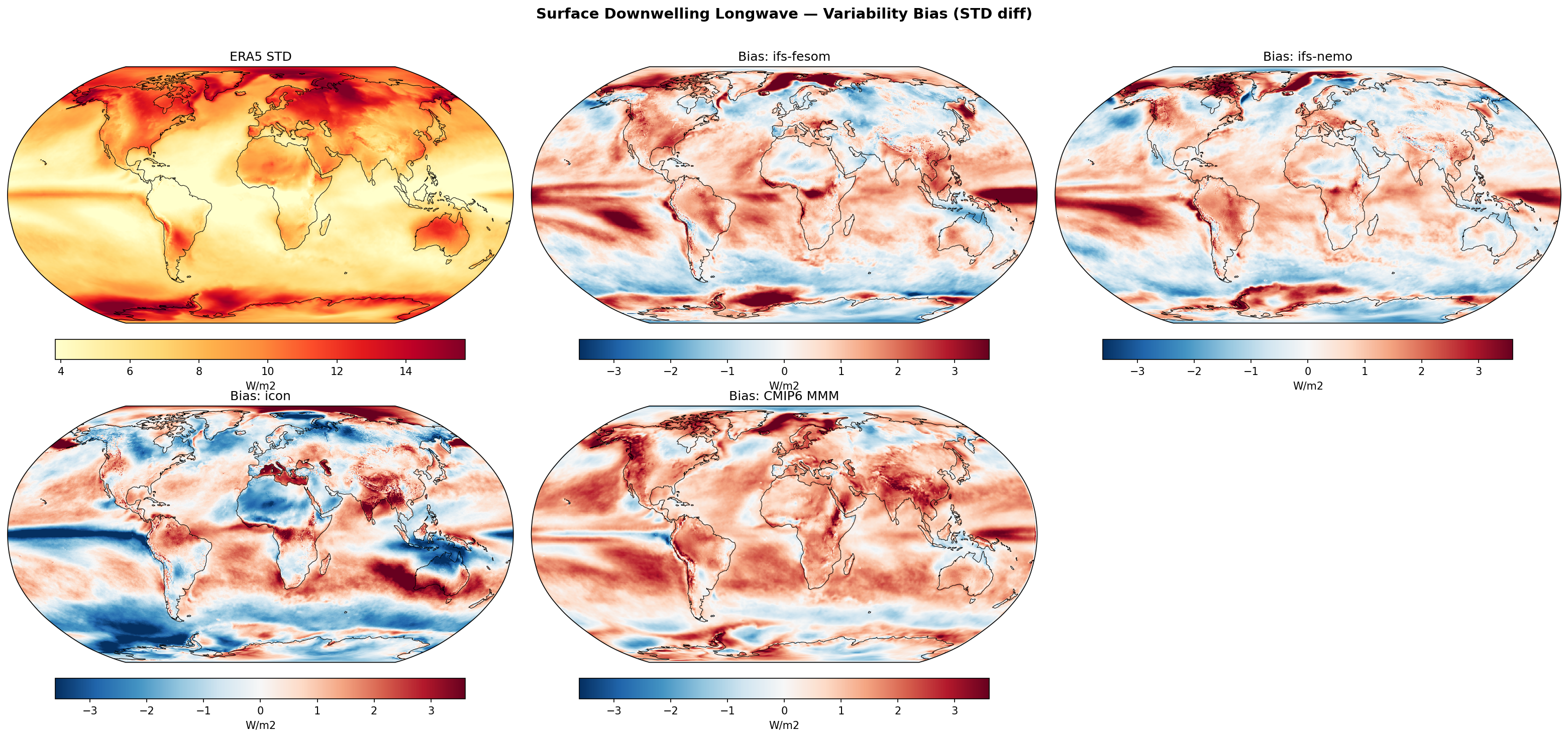
This figure evaluates the variability (standard deviation of anomalies) of surface downwelling longwave radiation (RLDS) in three high-resolution models compared to ERA5 reanalysis. The IFS-based models exhibit excessive variability in tropical convective regions, while ICON displays a distinct pattern of underestimated variability over oceans and overestimated variability over arid land masses.

Key Findings

IFS-FESOM and IFS-NEMO share a distinct bias pattern: excessive variability (positive bias >3 W/m²) in the tropical ITCZ/SPC and Amazon, likely linked to intermittent convective cloudiness.
ICON shows a strong land-sea contrast: it underestimates variability over most oceans (particularly the Tropical Atlantic and Southern Ocean) but overestimates it over arid/semi-arid land regions (Australia, North Africa, Mediterranean).
All three DestinE models underestimate RLDS variability in the Southern Ocean storm track, a region where ERA5 shows high intrinsic variability.
Despite having the lowest global mean bias (0.05 W/m²), ICON has the highest RMSE (1.55 W/m²), indicating that its small mean bias results from the cancellation of large opposing regional errors.
CMIP6 MMM shows a systematic positive bias across most of the globe, indicating that the conventional-resolution ensemble generally simulates more RLDS variability than ERA5.

Spatial Patterns

ERA5 shows peak variability in mid-latitude storm tracks and land masses. The IFS models capture the land patterns reasonably well but exaggerate tropical signals. ICON's spatial pattern is nearly inverted relative to the others in the tropics, showing widespread negative bias over oceans (too stable) and positive bias over dry lands.

Model Agreement

IFS-FESOM and IFS-NEMO are highly correlated in their bias structures, reflecting their shared atmospheric component. ICON diverges significantly, particularly in the sign of the bias over the tropical oceans. IFS-NEMO performs best overall in terms of RMSE (1.10 W/m²).

Physical Interpretation

RLDS variability is primarily driven by fluctuations in cloud cover (cloud radiative effect) and lower tropospheric temperature/humidity. The positive tropical bias in IFS models suggests 'on-off' convective behavior, creating large swings in cloudiness. ICON's negative oceanic bias suggests overly persistent cloud decks or dampened synoptic variability in the marine boundary layer. The high variability over arid lands in ICON suggests excessive surface temperature fluctuations or issues with clear-sky emissivity variance.

Caveats

ERA5 is a reanalysis product; its own cloud parameterizations influence the reference variability, particularly in data-sparse regions like the Southern Ocean.
The analysis assumes data is effectively deseasonalized; residual seasonal cycles could influence variability metrics in transition zones.

Surface Net Longwave Radiation — Variability (STD)

Variables	rls
Models	ifs-fesom, ifs-nemo, icon
Reference Dataset	ERA5
Units	W/m2
Period	1990–2014
ifs-fesom	Std Gmean: 5.74 · Diff Gmean: 0.17 · Rmse: 1.04
ifs-nemo	Std Gmean: 5.72 · Diff Gmean: 0.15 · Rmse: 0.92
icon	Std Gmean: 6.27 · Diff Gmean: 0.70 · Rmse: 1.79

Summary high

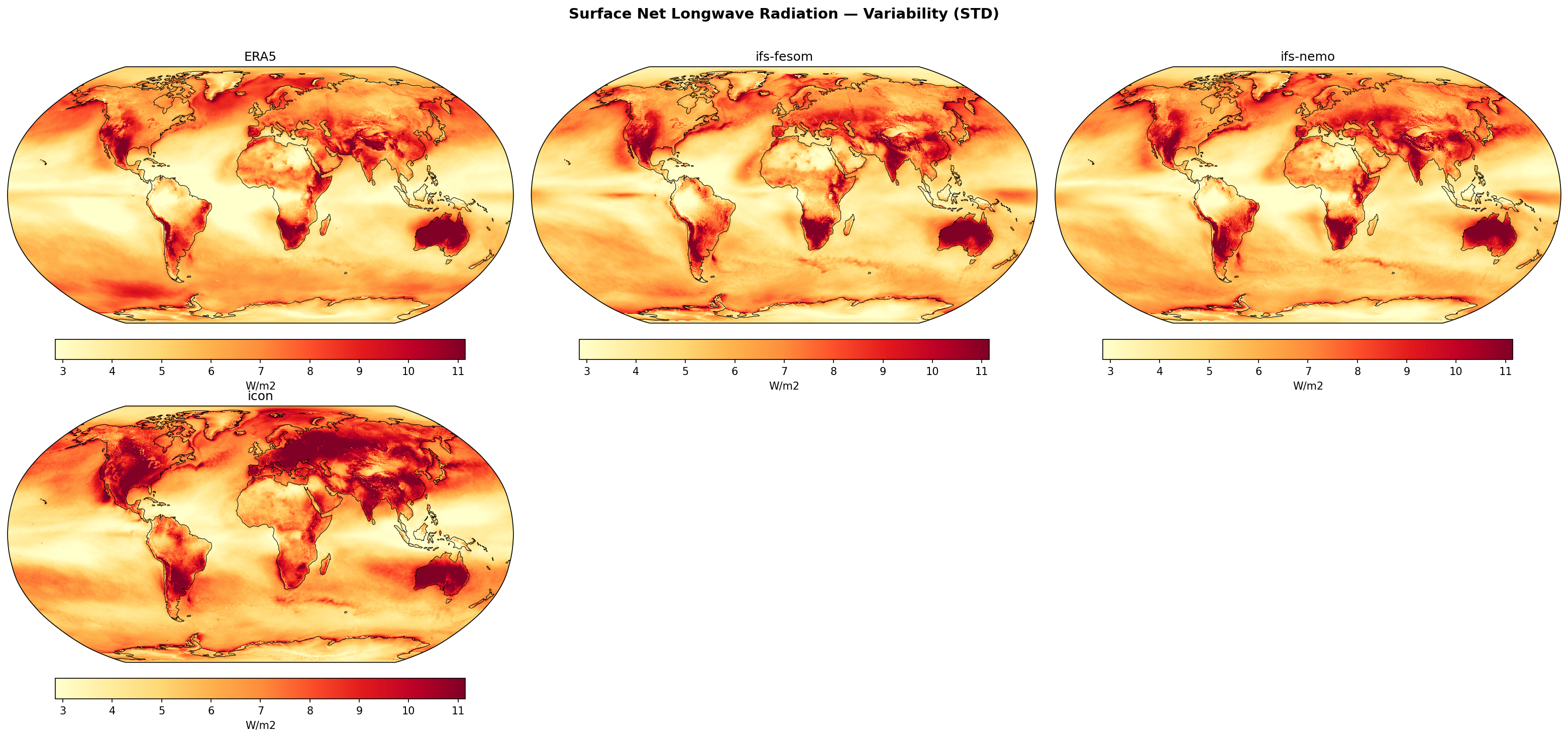
This diagnostic displays the standard deviation of deseasonalised, detrended monthly Surface Net Longwave Radiation for the period 1990–2014, comparing three high-resolution models (ifs-fesom, ifs-nemo, icon) against ERA5 reanalysis.

Key Findings

A strong land-sea contrast dominates the variability patterns, with continental interiors exhibiting much higher variability (>10 W/m²) than the oceans (<6 W/m²).
ifs-nemo and ifs-fesom show excellent agreement with ERA5 in both spatial pattern and magnitude, with low global-mean biases (+0.15–0.17 W/m²) and RMSEs (~0.9–1.0 W/m²).
icon systematically overestimates surface net longwave variability globally (global mean +0.7 W/m² relative to ERA5), with particularly intense variability over Northern Hemisphere land masses and tropical oceans.

Spatial Patterns

High variability is concentrated over major continental land masses (North America, Eurasia, South America, Australia) and oceanic storm tracks (North Atlantic, Southern Ocean), reflecting synoptic-scale fluctuations in temperature and cloud cover. Low variability characterizes the subtropical ocean gyres. The models generally reproduce the ERA5 features, including the bands of variability associated with the ITCZ and the contrast between arid (e.g., Sahara, slightly lower variance) and vegetated/transitional zones.

Model Agreement

The two IFS-based models (ifs-fesom and ifs-nemo) are nearly indistinguishable from each other and align closely with ERA5, suggesting that the choice of ocean model (unstructured FESOM vs structured NEMO) has minimal impact on surface longwave variability at this resolution. In contrast, icon is a distinct outlier, displaying excessive variability (higher standard deviation) across almost all regions, most notably over Eurasia and North America where the map is visibly saturated with high values (>11 W/m²).

Physical Interpretation

Surface net longwave variability is driven by fluctuations in surface skin temperature (dominant over land due to low heat capacity) and downwelling longwave radiation (driven by atmospheric temperature, water vapor, and cloud cover). The high variability over land in all plots reflects the rapid response of land surface temperature to synoptic forcing. ICON's overestimation likely stems from differences in its land surface coupling or cloud variability parameterizations, leading to larger fluctuations in surface temperature or cloud radiative effects compared to the IFS models and ERA5.

Caveats

The analysis relies on monthly means, which smooths out higher-frequency synoptic variability that might show different characteristics.
Potential observational uncertainties in ERA5 surface fluxes over data-sparse regions (e.g., Southern Ocean, interiors of Africa/South America) should be considered.

Surface Net Longwave Radiation — Variability Bias (STD diff)

Variables	rls
Models	ifs-fesom, ifs-nemo, icon
Reference Dataset	ERA5
Units	W/m2
Period	1990–2014
ifs-fesom	Std Gmean: 5.74 · Diff Gmean: 0.17 · Rmse: 1.04
ifs-nemo	Std Gmean: 5.72 · Diff Gmean: 0.15 · Rmse: 0.92
icon	Std Gmean: 6.27 · Diff Gmean: 0.70 · Rmse: 1.79

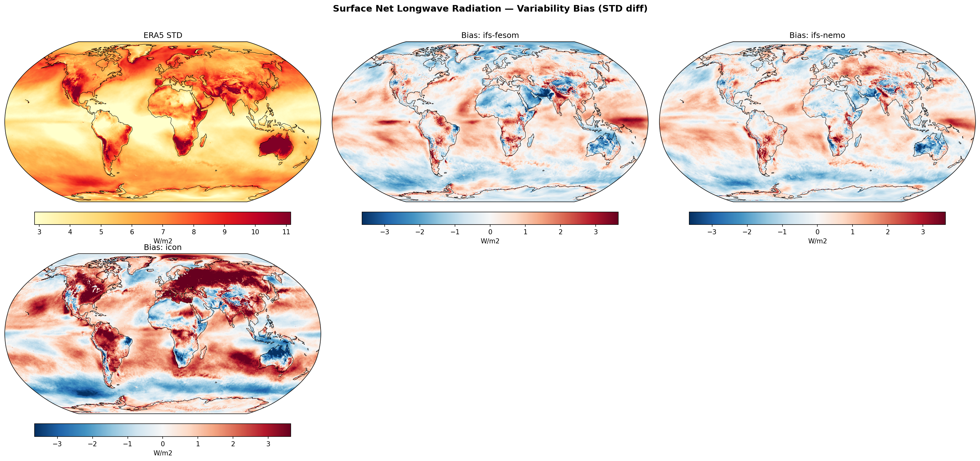
Summary high

This diagnostic evaluates the temporal variability (standard deviation) of Surface Net Longwave Radiation in three high-resolution models against ERA5 reanalysis. While the IFS-based models closely track ERA5 patterns, ICON exhibits a systematic overestimation of variability, particularly over continental landmasses.

Key Findings

ICON significantly overestimates variability globally (RMSE ~1.79 W/m²), with pronounced positive biases over all major land masses and the tropical oceans.
IFS-based models (ifs-fesom, ifs-nemo) show strong inter-model agreement and lower error metrics (RMSE ~0.9-1.0 W/m²), sharing similar bias patterns likely inherent to the IFS atmospheric physics.
All three models underestimate variability in the Southern Ocean (circumpolar negative bias) and North Atlantic storm track, indicating a potential common deficiency in capturing the variance of cloud radiative effects in these regimes.
Positive variability biases are concentrated along the ITCZ and SPCZ in the tropical Pacific for all models, suggesting excessive intermittency in convective cloud cover.

Spatial Patterns

ERA5 shows peak variability over Northern Hemisphere continents and tropical convergence zones. The models generally reproduce this morphology, but amplitude differences are striking. ICON paints land regions in deep red (excess variability > 2-3 W/m²), whereas the IFS models show patchier, weaker positive biases. The Southern Ocean appears as a consistent band of underestimated variability (blue) in all simulations, most intense in ICON.

Model Agreement

There is very high agreement between ifs-fesom and ifs-nemo, confirming that surface longwave variability is primarily driven by the atmospheric component (which they share) rather than the ocean model formulation. ICON stands out as an outlier with significantly higher variance.

Physical Interpretation

Surface Net Longwave variability is driven by surface temperature fluctuations and changes in downwelling atmospheric radiation (clouds/water vapour). The excessive land variability in ICON suggests over-responsive surface temperatures (potentially linked to land-surface coupling or thermal inertia in the JSBACH component) or overly intermittent cloud cover. The pervasive underestimation of variability in the Southern Ocean implies that modeled cloud decks in this region may be too persistent or uniform, lacking the temporal dynamism (e.g., frontal clearing) seen in ERA5.

Caveats

ERA5 surface fluxes are generated by the IFS model (Cy41r2), creating an expected kinship with the ifs-nemo and ifs-fesom results; ICON is penalized for using a different physical formulation.
This diagnostic measures the standard deviation of fluctuations, not the mean state; models could have correct variability but incorrect mean values.

Surface Net Longwave Radiation (Clear-Sky) — Variability (STD)

Variables	rlscs
Models	ifs-fesom, ifs-nemo, icon
Reference Dataset	ERA5
Units	W/m2
Period	1990–2014
ifs-fesom	Std Gmean: 4.58 · Diff Gmean: 0.44 · Rmse: 1.08
ifs-nemo	Std Gmean: 4.41 · Diff Gmean: 0.26 · Rmse: 0.84
icon	Std Gmean: 4.52 · Diff Gmean: 0.37 · Rmse: 1.40

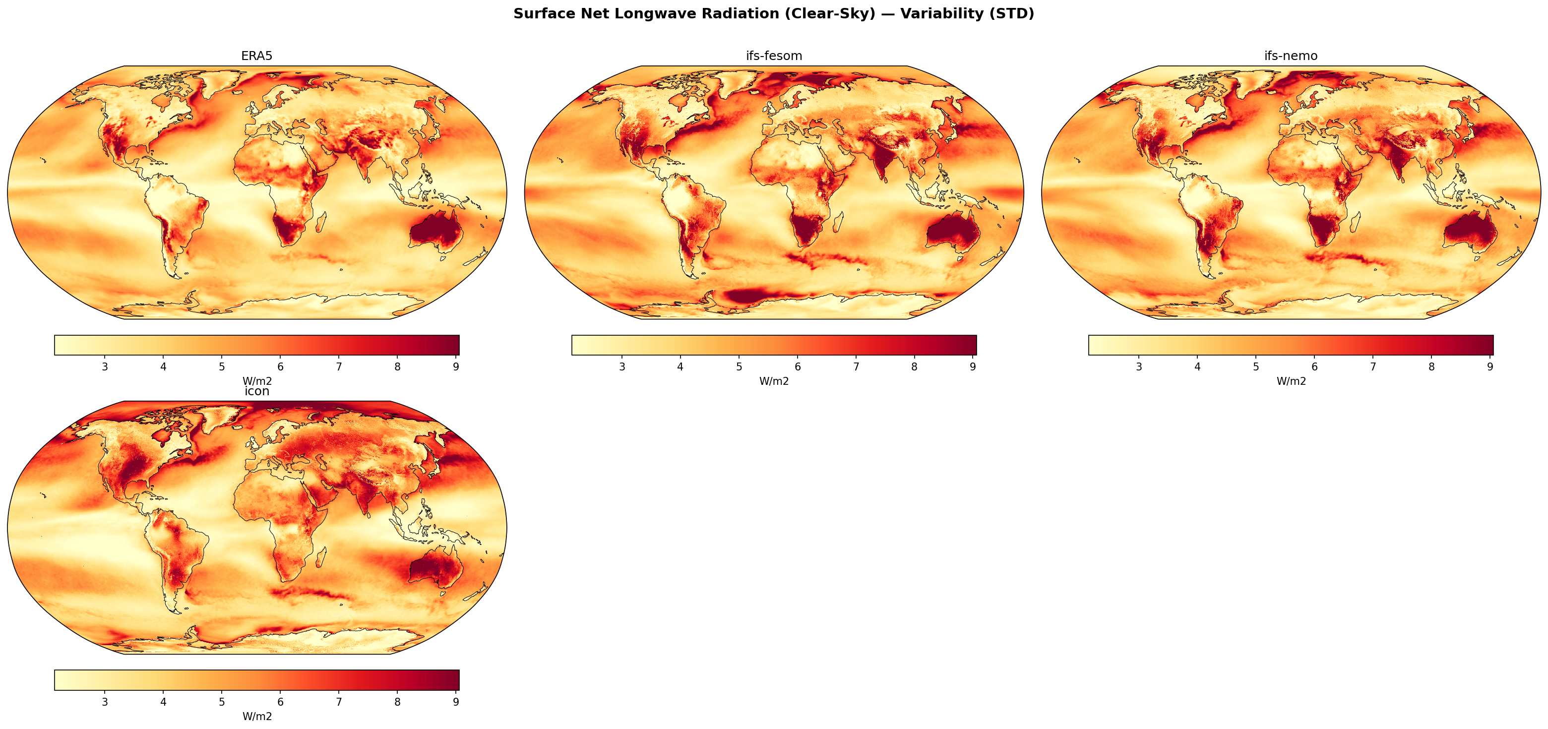
Summary high

This diagnostic shows the standard deviation of clear-sky surface net longwave radiation, highlighting regions where surface temperature and atmospheric moisture fluctuate most strongly. The models generally reproduce the observed contrast between high-variability land masses and low-variability oceans, though all three overestimate the global mean variability relative to ERA5.

Key Findings

High variability (>8 W/m²) is observed over arid and semi-arid land regions (e.g., Australia, Sahara, Western US) and Western Boundary Currents, driven by surface temperature fluctuations.
ifs-nemo shows the best agreement with ERA5, having the lowest RMSE (0.84 W/m²) and the smallest positive bias (+0.26 W/m²) in global mean variability.
ifs-fesom exhibits a distinct region of excessive variability in the Atlantic sector of the Southern Ocean (Weddell Sea area) which is not present in ERA5 or the other models.
icon captures the general spatial structure but has the highest RMSE (1.40 W/m²), indicating larger regional mismatches in variability amplitude compared to the IFS-based models.

Spatial Patterns

Variability is dominated by a strong land-sea contrast. Over land, low thermal inertia leads to high surface temperature variance and thus high LW variability, particularly in dry regions where atmospheric damping is weak. Over oceans, variability peaks in the Gulf Stream and Kuroshio extensions (associated with SST fronts) and high latitudes. Tropical oceans display the lowest variability.

Model Agreement

All models capture the primary terrestrial and western boundary current features well. Disagreement is most pronounced in the high-latitude Southern Ocean, where ifs-fesom shows significantly higher variability than ifs-nemo, icon, or ERA5. The two IFS variants are visually closer to each other than to ICON, particularly in the sharpness of storm track features.

Physical Interpretation

Clear-sky surface net longwave variability is governed by fluctuations in surface skin temperature ($T_{skin}$) and near-surface humidity. Land areas with low heat capacity respond strongly to synoptic weather, driving high $T_{skin}$ variability. In the Southern Ocean, the discrepancy in ifs-fesom likely arises from highly variable sea ice concentrations or open-ocean convection events (polynyas) that drastically alter surface temperatures and air-sea fluxes compared to the reanalysis.

Caveats

ERA5 reanalysis relies on assimilated data which is sparser in the Southern Ocean, potentially making the 'observed' low variability there less certain.
Clear-sky diagnostics exclude cloud effects, meaning total radiative variability (including clouds) would likely show different patterns, particularly in storm tracks.

Surface Net Longwave Radiation (Clear-Sky) — Variability Bias (STD diff)

Variables	rlscs
Models	ifs-fesom, ifs-nemo, icon
Reference Dataset	ERA5
Units	W/m2
Period	1990–2014
ifs-fesom	Std Gmean: 4.58 · Diff Gmean: 0.44 · Rmse: 1.08
ifs-nemo	Std Gmean: 4.41 · Diff Gmean: 0.26 · Rmse: 0.84
icon	Std Gmean: 4.52 · Diff Gmean: 0.37 · Rmse: 1.40

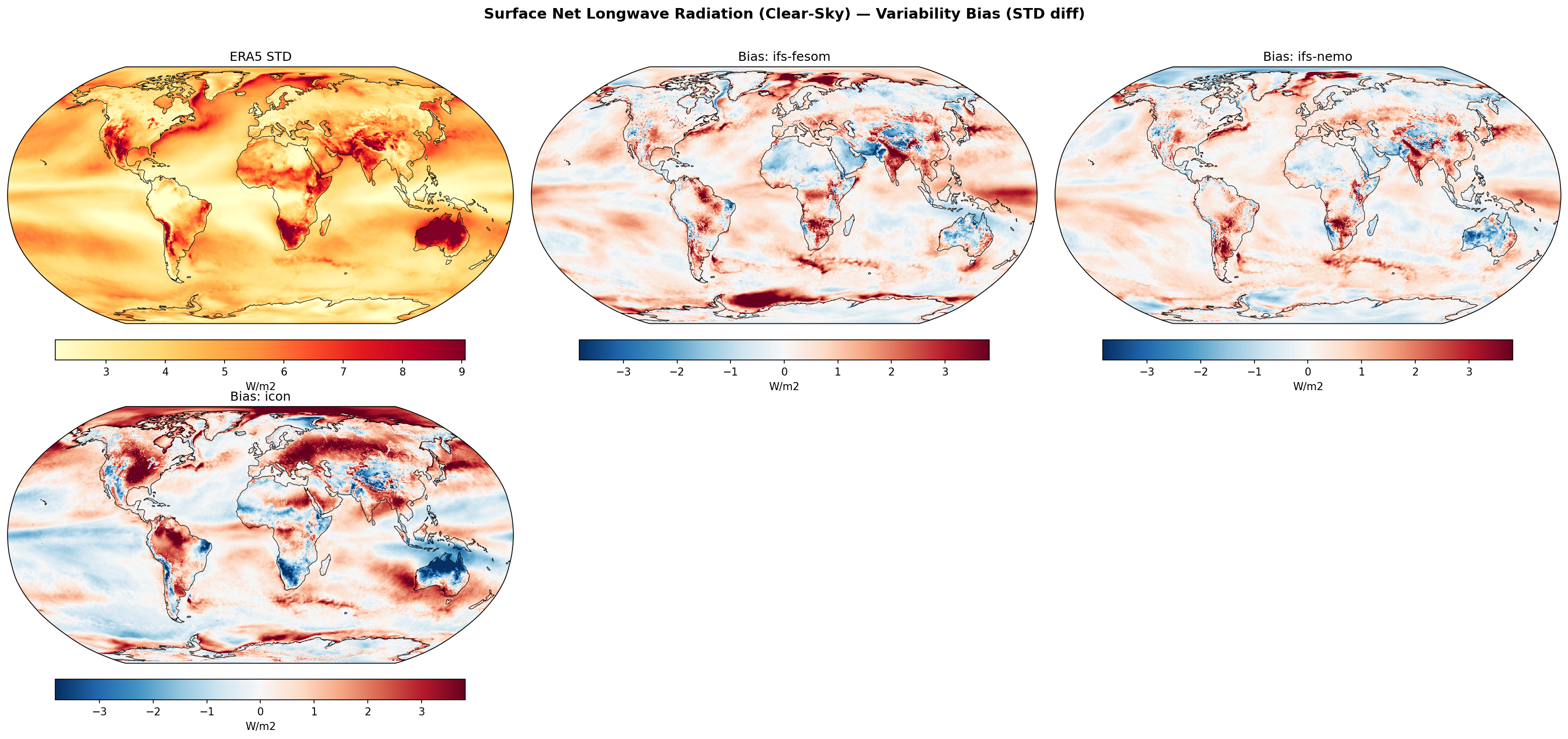
Summary high

This figure evaluates the variability (standard deviation) of clear-sky surface net longwave radiation in three high-resolution coupled models against ERA5 reanalysis. While IFS-based models (IFS-FESOM and IFS-NEMO) show similar bias patterns with moderate overestimation in the extratropics, ICON exhibits a distinct behavior with excessive variability over land and suppressed variability over tropical oceans.

Key Findings

IFS-NEMO demonstrates the best agreement with observations (RMSE 0.84 W/m²), closely followed by IFS-FESOM, indicating the stability of the IFS atmospheric component across different ocean couplings.
ICON displays a strong systematic bias contrast: it significantly overestimates variability over extratropical continents (biases > +3 W/m²) while underestimating it over most tropical and subtropical oceans.
All models exhibit a negative variability bias (underestimation) over key tropical rainforest regions (Amazon, Congo) and the Indo-Pacific Warm Pool, suggesting a dampening of clear-sky radiative variance in deep convective zones.
A localized region of extreme positive bias exists in the Weddell Sea sector of the Southern Ocean, particularly pronounced in IFS-FESOM, likely linked to sea-ice variability differences between FESOM and NEMO.

Spatial Patterns

ERA5 shows peak variability (7-9 W/m²) over arid and semi-arid land regions (Sahara, Australia, Western US), driven by strong diurnal and synoptic surface temperature fluctuations. The models generally capture this land-sea contrast. However, IFS models show patchy positive biases in the Southern Ocean storm tracks and high mountain ranges (Himalayas, Andes). ICON's spatial pattern is dominated by a hemispheric split: widespread positive biases over Northern Hemisphere landmasses and negative biases over lower-latitude oceans.

Model Agreement

There is high agreement between IFS-FESOM and IFS-NEMO, confirming that the atmospheric model primarily dictates surface radiation variability, though the choice of ocean/ice model modulates this in polar regions (e.g., Weddell Sea). ICON diverges significantly from the IFS group, particularly in its land surface response.

Physical Interpretation

Variability in clear-sky surface net longwave radiation is primarily driven by skin temperature fluctuations ($T_{skin}$) and near-surface humidity/temperature variations (affecting $LW_{down}$). The excessive variability in ICON over land suggests that its land surface scheme may have lower thermal inertia or stronger coupling to atmospheric drying than ERA5, leading to larger swings in $T_{skin}$. Conversely, the negative biases in the tropics across all models suggest they may lack the episodic dry intrusions or specific synoptic variability found in ERA5, resulting in a more persistent, less variable radiative regime. The Southern Ocean biases likely relate to dynamic sea-ice variability affecting surface emission.

Caveats

Differences in clear-sky sampling definitions between models and reanalysis can introduce biases.
ERA5 variability includes assimilation increments, which can inject variance that free-running models are not expected to reproduce exactly.

TOA Net Longwave Radiation — Variability (STD)

Variables	rlt
Models	ifs-fesom, ifs-nemo, icon
Reference Dataset	ERA5
Units	W/m2
Period	1990–2014
ifs-fesom	Std Gmean: 8.45 · Diff Gmean: 0.59 · Rmse: 1.88
ifs-nemo	Std Gmean: 8.35 · Diff Gmean: 0.49 · Rmse: 1.64
icon	Std Gmean: 7.22 · Diff Gmean: -0.64 · Rmse: 2.47

Summary high

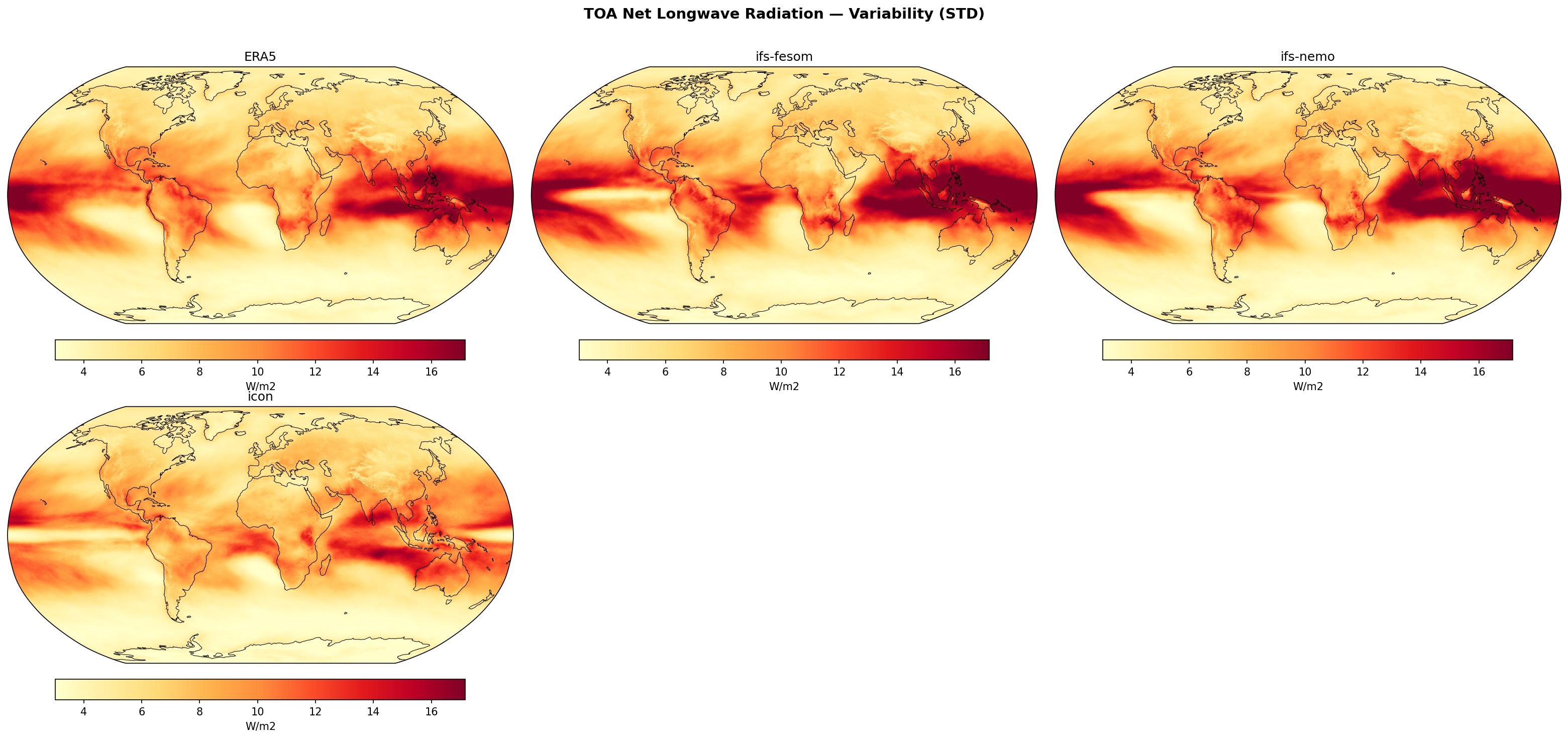
This diagnostic shows the standard deviation of deseasonalised, detrended TOA Net Longwave Radiation (1990–2014), serving as a proxy for the variability of deep convection and cloud radiative effects.

Key Findings

All models successfully reproduce the major spatial centers of longwave variability, specifically the Indo-Pacific Warm Pool, the Intertropical Convergence Zone (ITCZ), and the South Pacific Convergence Zone (SPCZ).
The IFS-based models (ifs-fesom and ifs-nemo) exhibit slightly higher variability than ERA5 (global mean bias ~+0.5 W/m²), particularly broadening the zones of high variability in the tropical Pacific.
ICON underestimates the variability intensity globally (bias -0.64 W/m²), showing notably weaker variance in the primary tropical convective regions compared to ERA5 and the IFS models.

Spatial Patterns

The dominant pattern is high variability (>14 W/m²) in the tropical convective belts (Warm Pool, ITCZ, SPCZ), driven by the intermittency of deep convection and cloud cover changes (e.g., ENSO-related shifts). Mid-latitudes show moderate variability associated with storm tracks, while subtropical subsidence zones and polar regions exhibit low variability (<6 W/m²).

Model Agreement

The two IFS variants are nearly identical, indicating the atmospheric model component dominates this metric. They agree well with ERA5 spatially but differ in magnitude. ICON captures the pattern structure but consistently underestimates the amplitude of the variability, resulting in the highest RMSE (2.47 W/m²) among the models.

Physical Interpretation

TOA Net Longwave variability in the tropics is primarily driven by fluctuations in cloud top height associated with deep convection. The high variability regions correspond to areas where convection is dynamic (e.g., responding to ENSO or MJO). The IFS models appear to have more energetic convective variability or stronger ENSO-related shifts, while ICON likely has more persistent cloud features or damped interannual variability in convective organization.

Caveats

Differences in land-sea masks or grid resolution may contribute to minor local discrepancies.
The analysis relies on ERA5 as truth; while robust for OLR due to satellite assimilation, it is still a reanalysis product.

TOA Net Longwave Radiation — Variability Bias (STD diff)

Variables	rlt
Models	ifs-fesom, ifs-nemo, icon
Reference Dataset	ERA5
Units	W/m2
Period	1990–2014
ifs-fesom	Std Gmean: 8.45 · Diff Gmean: 0.59 · Rmse: 1.88
ifs-nemo	Std Gmean: 8.35 · Diff Gmean: 0.49 · Rmse: 1.64
icon	Std Gmean: 7.22 · Diff Gmean: -0.64 · Rmse: 2.47

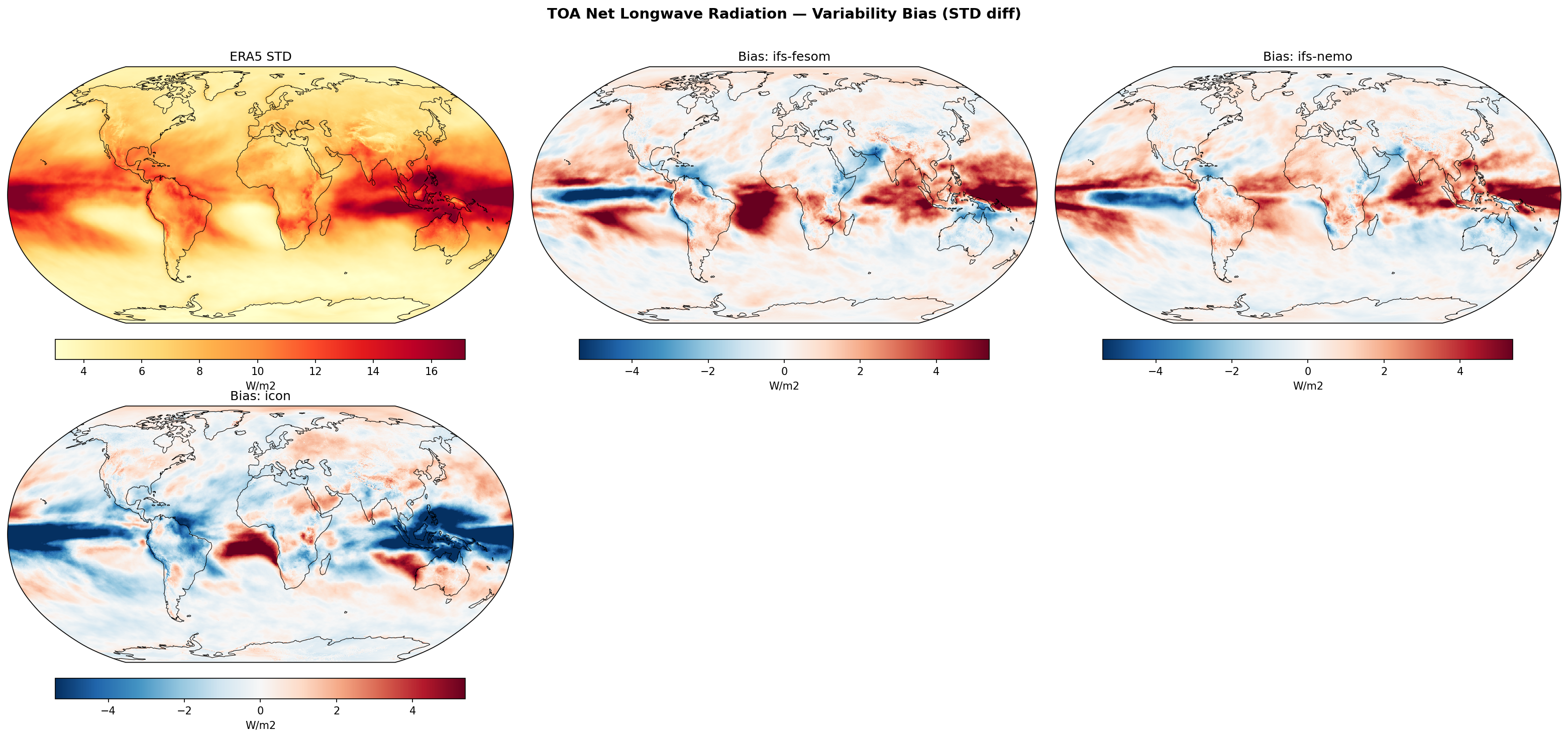
Summary high

This figure evaluates the variability (standard deviation of anomalies) of Top-of-Atmosphere Net Longwave Radiation across three high-resolution models compared to ERA5. The IFS-based models generally overestimate variability in the Indo-Pacific Warm Pool and tropical land masses while underestimating it in the ITCZ bands, whereas ICON exhibits a systematic underestimation of variability across most tropical oceans.

Key Findings

IFS-FESOM and IFS-NEMO share a distinct spatial bias pattern: excessive variability (>4 W/m²) over the Maritime Continent, South America, and Africa, contrasted with underestimated variability in the central/eastern Pacific and Atlantic ITCZ.
ICON displays a widespread negative bias (underestimation) of variability over the tropical oceans, particularly within the ITCZ and SPCZ, leading to the highest RMSE (2.47 W/m²) and a negative global mean bias (-0.64 W/m²).
IFS-NEMO performs best statistically (RMSE 1.64 W/m²), closely followed by IFS-FESOM, indicating that the atmospheric component (IFS) rather than the ocean model primarily dictates TOA radiation variability errors.
ERA5 shows peak variability in the convective zones (ITCZ, SPCZ, tropical land); models generally struggle to reproduce the correct magnitude of this variance, either suppressing it (ICON oceans) or exaggerating its localization (IFS Warm Pool).

Spatial Patterns

The most prominent features are the zonal bands of negative bias in the ITCZ regions (Atlantic and Pacific) seen in all models, though most severe in ICON. IFS models show a strong dipole in the Pacific: positive bias in the west (Warm Pool) and negative in the central/east. All models show positive biases over tropical continents (Amazon, Congo Basin).

Model Agreement

IFS-FESOM and IFS-NEMO show high agreement in their spatial bias structures, confirming the dominance of atmospheric physics. ICON diverges significantly, producing much lower variability over oceans than the IFS family.

Physical Interpretation

TOA Net Longwave variability in the tropics is driven by fluctuations in cloud top height and deep convection (OLR). The positive biases over land and the Warm Pool in IFS suggest overly intermittent or intense deep convection. The negative biases in the ITCZ (especially in ICON) suggest a 'locked' ITCZ with insufficient meridional fluctuation or overly persistent, non-variable cloud cover compared to the episodic nature of real convection. The distinct land-sea contrast in bias indicates different convective parameterisation sensitivities to surface forcing.

Caveats

ERA5 TOA radiation is a reanalysis product and relies on its own radiative transfer model, though constrained by assimilation; direct comparison with CERES for variability would be a stricter test.
The analysis does not distinguish between timescales (e.g., ENSO vs. MJO vs. synoptic), so biases could stem from errors in specific variability modes.

TOA Net Longwave Radiation (Clear-Sky) — Variability (STD)

Variables	rltcs
Models	ifs-fesom, ifs-nemo, icon
Reference Dataset	ERA5
Units	W/m2
Period	1990–2014
ifs-fesom	Std Gmean: 3.56 · Diff Gmean: 0.28 · Rmse: 0.65
ifs-nemo	Std Gmean: 3.44 · Diff Gmean: 0.17 · Rmse: 0.47
icon	Std Gmean: 3.14 · Diff Gmean: -0.13 · Rmse: 0.73

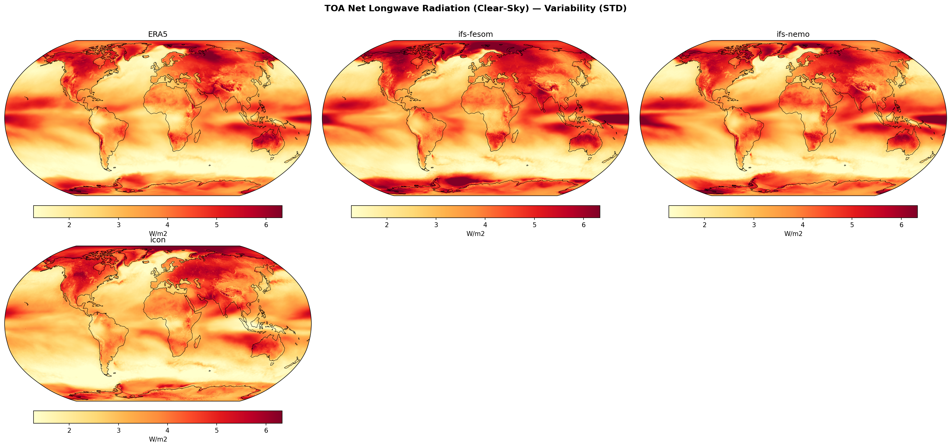
Summary high

This diagnostic evaluates the interannual variability (standard deviation) of clear-sky outgoing longwave radiation (OLR), highlighting regions dominated by surface temperature and water vapor fluctuations such as the ENSO region and high latitudes.

Key Findings

All models capture the primary variability hotspots: the tropical Pacific (ENSO), Northern Hemisphere continental interiors, and the Southern Ocean sea-ice zone.
IFS-based models (ifs-fesom, ifs-nemo) reproduce the strong ENSO variability signature in the Pacific well, though ifs-fesom tends to slightly overestimate global variability (+0.28 W/m² bias).
ICON significantly underestimates variability in the tropical Pacific, showing a much weaker ENSO signature compared to ERA5 and the IFS models, contributing to a negative global mean bias (-0.13 W/m²).

Spatial Patterns

Dominant spatial features include a tongue of high variability (>5 W/m²) extending from the South American coast into the central Pacific (ENSO), high variability over NH land masses (Siberia, North America) due to large surface temperature variance, and a band over the Southern Ocean driven by sea-ice edge variability.

Model Agreement

ifs-nemo shows the best agreement with ERA5 (lowest RMSE of 0.47 W/m² and smallest bias). ifs-fesom is structurally similar but more energetic. ICON diverges most significantly in the tropics, appearing 'washed out' compared to the observational baseline.

Physical Interpretation

Clear-sky OLR variability is primarily driven by Surface Temperature (Stefan-Boltzmann law) and column water vapor changes. The high variability in the Pacific corresponds to interannual SST fluctuations associated with ENSO (El Niño/La Niña). The muted signal in ICON suggests either damped SST variability (weak ENSO amplitude) or differences in the water vapor feedback relative to the IFS models. High-latitude variability tracks surface temperature extremes over land and sea-ice variations.

Caveats

This diagnostic shows clear-sky fluxes only; total OLR variability would include cloud radiative effects which often dampen clear-sky signals in the tropics.
Differences in land surface schemes (temperature variance) may contribute to discrepancies over continents.

TOA Net Longwave Radiation (Clear-Sky) — Variability Bias (STD diff)

Variables	rltcs
Models	ifs-fesom, ifs-nemo, icon
Reference Dataset	ERA5
Units	W/m2
Period	1990–2014
ifs-fesom	Std Gmean: 3.56 · Diff Gmean: 0.28 · Rmse: 0.65
ifs-nemo	Std Gmean: 3.44 · Diff Gmean: 0.17 · Rmse: 0.47
icon	Std Gmean: 3.14 · Diff Gmean: -0.13 · Rmse: 0.73

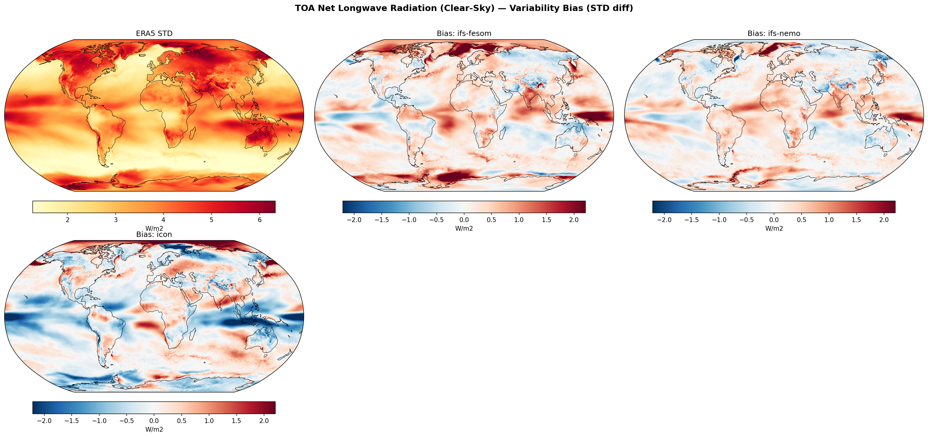
Summary high

This diagnostic evaluates the variability (standard deviation) of clear-sky TOA net longwave radiation. The ifs-nemo model shows the best agreement with ERA5, while ifs-fesom generally overestimates variability and icon displays a marked contrast between suppressed oceanic and enhanced continental variability.

Key Findings

All models exhibit strong excess variability (>1.5 W/m²) over Antarctica, Greenland, and the Himalayas compared to ERA5.
ifs-nemo achieves the lowest global RMSE (0.47 W/m²) and bias, while ifs-fesom shows a similar spatial pattern but with higher magnitude positive biases (RMSE 0.65 W/m²).
icon shows a distinct systematic negative bias (suppressed variability) over most tropical and temperate oceans, particularly in the Pacific and Atlantic basins.

Spatial Patterns

ERA5 shows peak variability over high-latitude land masses and the Warm Pool. The models consistently overestimate variability over ice sheets and high orography. ifs-fesom and ifs-nemo show scattered positive biases in the tropics, whereas icon shows coherent bands of negative bias in the ITCZ/SPCZ regions and broader oceans, contrasting with its positive bias over Northern Hemisphere land.

Model Agreement

The two IFS-based models (ifs-fesom and ifs-nemo) show high structural agreement, suggesting the atmospheric model physics dominates the pattern, though the ocean coupling (FESOM vs NEMO) modulates the amplitude. ICON diverges significantly in its treatment of oceanic variability.

Physical Interpretation

Since this is clear-sky radiation, variability is driven by surface temperature (Ts) and column water vapor. The excess variability over land and ice sheets suggests models may have overly responsive surface skin temperatures or issues with stable boundary layer decoupling in polar night. ICON's reduced oceanic variability implies damped fluctuations in either sea surface temperatures or, more likely, tropospheric humidity compared to ERA5.

Caveats

Clear-sky fluxes are diagnostic calculations; discrepancies may partly arise from differences in radiative transfer schemes versus the ERA5 assimilation system.
The strong biases over high orography may be influenced by resolution differences in topographic representation between the 5km models and the ERA5 grid.

Surface Downwelling Shortwave — Variability (STD)

Variables	rsds
Models	ifs-fesom, ifs-nemo, icon, CMIP6 MMM
Reference Dataset	ERA5
Units	W/m2
Period	1990–2014
ifs-fesom	Std Gmean: 12.66 · Diff Gmean: 0.90 · Rmse: 2.43
ifs-nemo	Std Gmean: 12.62 · Diff Gmean: 0.86 · Rmse: 2.20
icon	Std Gmean: 11.96 · Diff Gmean: 0.20 · Rmse: 3.38
CMIP6 MMM	Std Gmean: 13.85 · Diff Gmean: 2.10 · Rmse: 2.90

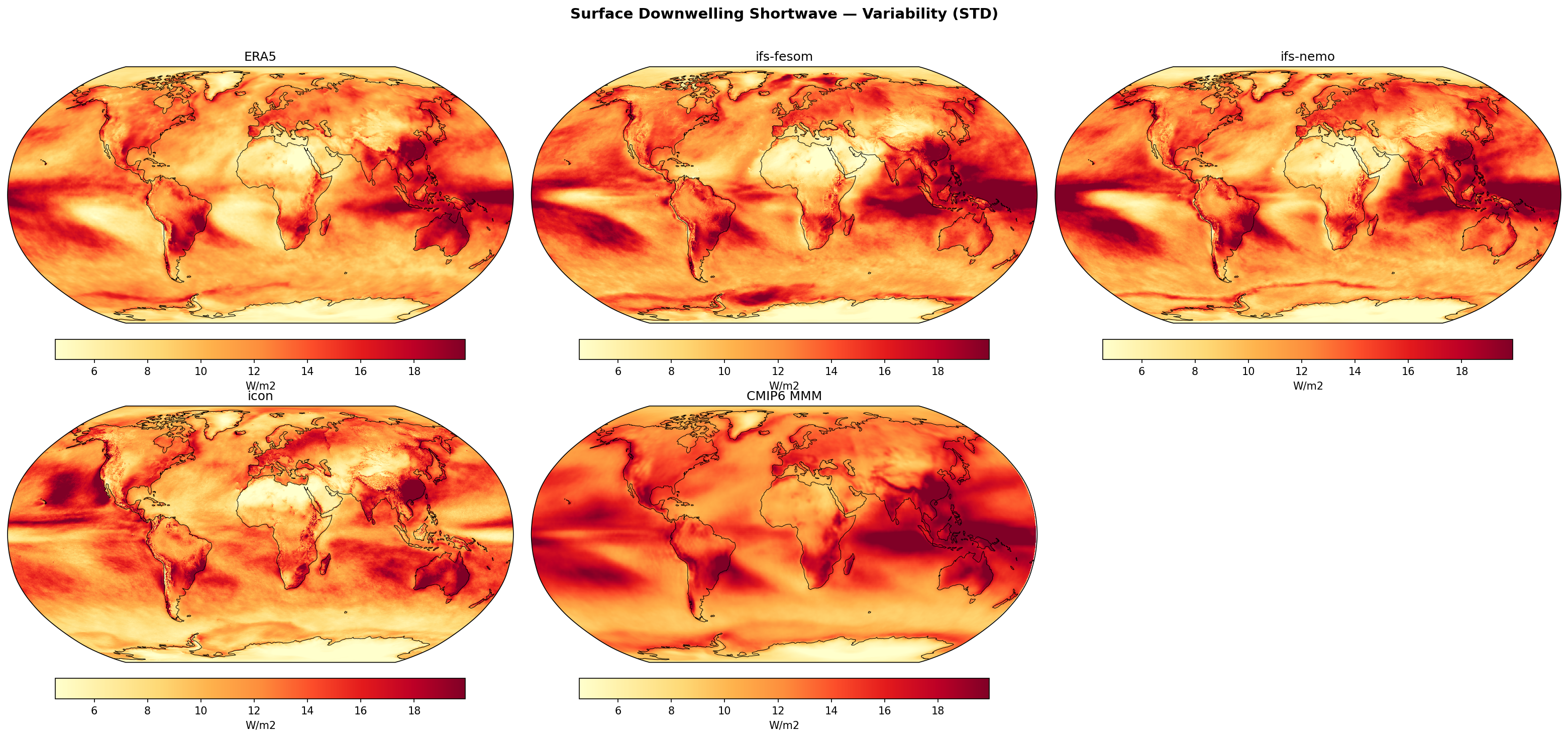
Summary high

This diagnostic evaluates the temporal variability (standard deviation) of surface downwelling shortwave radiation (RSDS) in DestinE models compared to ERA5 and CMIP6. The IFS-based models capture the spatial structure of variability accurately but overestimate its magnitude, whereas ICON exhibits lower overall bias but significant spatial errors in the tropical Pacific.

Key Findings

IFS-NEMO and IFS-FESOM demonstrate superior spatial fidelity (RMSE ~2.2-2.4 W/m²) compared to ICON (RMSE ~3.4 W/m²) and CMIP6 (RMSE ~2.9 W/m²), reproducing the observed patterns of variability in the ENSO region and storm tracks.
All models tend to overestimate the magnitude of SW variability globally relative to ERA5, with CMIP6 MMM showing the largest positive bias (+2.1 W/m²) and IFS models showing moderate positive bias (~+0.9 W/m²).
ICON presents a distinct spatial anomaly in the eastern Tropical Pacific, showing a concentrated 'bullseye' of extreme variability rather than the broader zonal patterns seen in ERA5 and IFS.
Variability over stratocumulus regions (e.g., off Peru/Chile, Namibia) is captured by all models but is generally more intense and spatially extended in the simulations than in ERA5.

Spatial Patterns

The dominant feature in all panels is high SW variability (>18 W/m²) in the tropical Pacific, associated with ENSO-driven cloud fluctuations. ERA5 shows a coherent tongue of variability extending from South America across the Pacific. IFS models reproduce this shape but with higher intensity. ICON fails to reproduce the continuous zonal structure, instead showing disjointed high-variability patches in the eastern Pacific and distinct artifacts over the Amazon. Over land, models generally show higher variability than ERA5, particularly in convective regions like Central Africa and South America.

Model Agreement

There is very strong agreement between IFS-FESOM and IFS-NEMO, indicating that the atmospheric physics (shared) rather than the ocean grid (distinct) dominates surface radiation variability. ICON diverges significantly from the IFS/ERA5 pattern, suggesting different cloud or convection parameterisation behaviour. The DestinE IFS models are closer to ERA5 in both magnitude and pattern than the CMIP6 Multi-Model Mean.

Physical Interpretation

Surface shortwave variability on monthly timescales is primarily driven by fluctuations in cloud fraction and optical depth. The general overestimation of variability in models suggests they may lack the persistence of cloud regimes seen in observations, switching too frequently between clear and cloudy states, or simulating overly optically thick clouds. ICON's specific issues in the tropical Pacific likely reflect biases in the ITCZ position or convective triggering (e.g., 'pop-corn' convection) that create unrealistic localized variance in cloud cover.

Caveats

ERA5 is a reanalysis product and relies on model physics for radiative transfer, though it assimilates satellite data; direct comparison with satellite products like CERES would confirm the baseline.
The CMIP6 MMM likely represents the mean of individual model standard deviations; the high value indicates that conventional-resolution models generally struggle to capture the stability of radiative regimes.

Surface Downwelling Shortwave — Variability Bias (STD diff)

Variables	rsds
Models	ifs-fesom, ifs-nemo, icon, CMIP6 MMM
Reference Dataset	ERA5
Units	W/m2
Period	1990–2014
ifs-fesom	Std Gmean: 12.66 · Diff Gmean: 0.90 · Rmse: 2.43
ifs-nemo	Std Gmean: 12.62 · Diff Gmean: 0.86 · Rmse: 2.20
icon	Std Gmean: 11.96 · Diff Gmean: 0.20 · Rmse: 3.38
CMIP6 MMM	Std Gmean: 13.85 · Diff Gmean: 2.10 · Rmse: 2.90

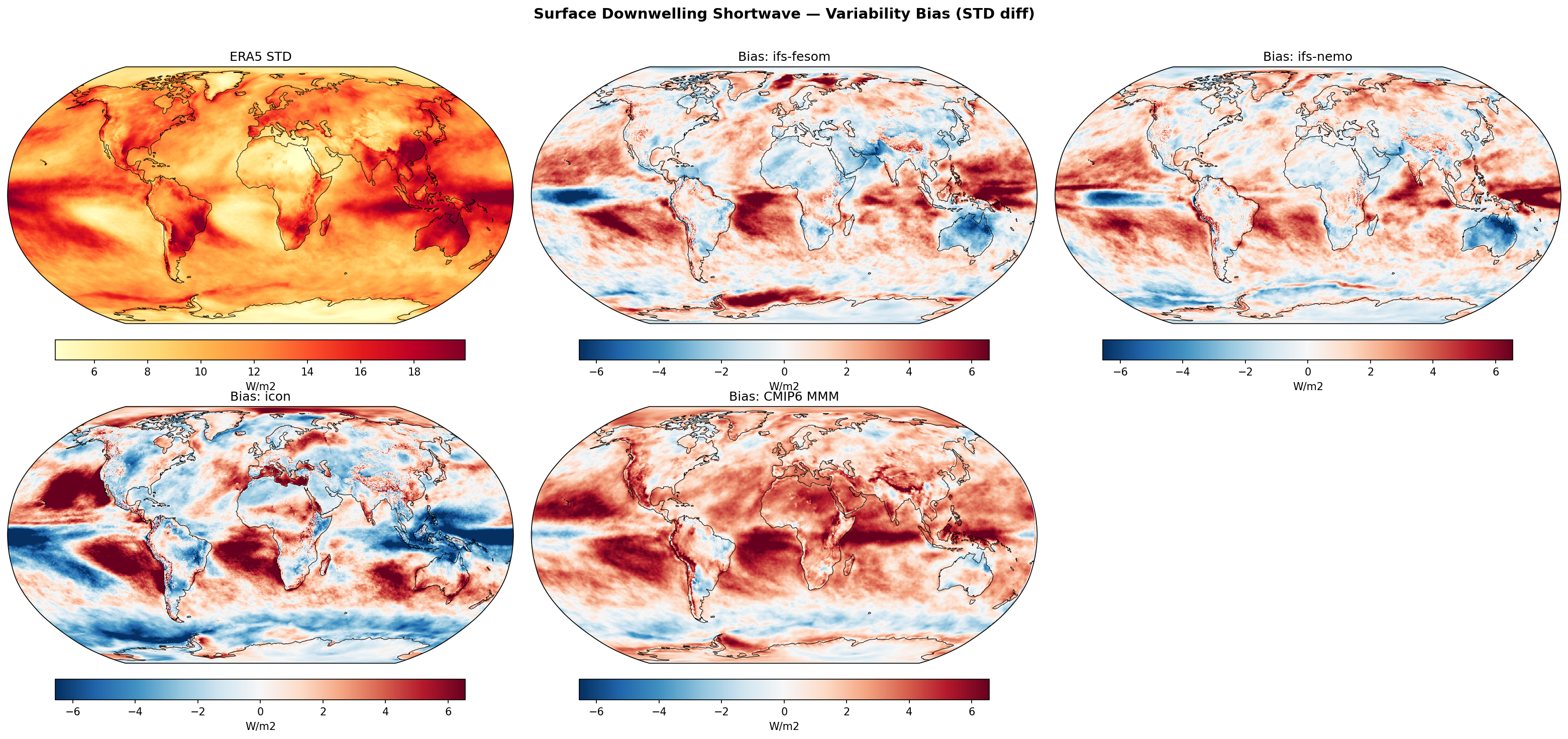
Summary high

This figure evaluates the variability (standard deviation) of surface downwelling shortwave radiation in DestinE models (IFS-FESOM, IFS-NEMO, ICON) and the CMIP6 multi-model mean against ERA5 reanalysis. While CMIP6 shows a systematic global overestimation of variability, the high-resolution models exhibit a regime-dependent bias structure with underestimated variability in deep convective zones and overestimated variability in subtropical subsidence regions.

Key Findings

IFS-NEMO and IFS-FESOM display very similar bias patterns, characterized by suppressed variability in the ITCZ (negative bias) and excess variability in subtropical stratocumulus and trade-wind regions (positive bias).
ICON exhibits the strongest spatial contrasts and highest RMSE (3.38 W/m²), with intense positive biases in the SE Pacific and SE Atlantic stratocumulus decks and strong negative biases in the tropical convective belts.
The CMIP6 Multi-Model Mean generally overestimates surface SW variability globally (mean bias +2.10 W/m²), whereas the high-resolution models have smaller global mean biases due to error cancellation between regions.
IFS-NEMO achieves the lowest spatial RMSE (2.20 W/m²) among the evaluated datasets, indicating the best agreement with ERA5 variability patterns.

Spatial Patterns

The dominant feature in the high-resolution models is a zonal contrast: negative bias (blue) in the equatorial Pacific and Indian Ocean deep convection zones, and positive bias (red) in the eastern ocean basins (subtropical highs) and mid-latitude storm tracks. ICON amplifies this pattern significantly compared to the IFS variants. In contrast, CMIP6 shows a pervasive positive bias across most of the globe, lacking the distinct equatorial suppression seen in the DestinE models.

Model Agreement

IFS-FESOM and IFS-NEMO show high agreement with each other, reflecting their shared atmospheric component. ICON diverges with significantly larger bias magnitudes, particularly in the Pacific ITCZ and eastern boundary upwelling regions. All high-res models disagree with the CMIP6 MMM, which lacks the strong negative tropical bias.

Physical Interpretation

The patterns suggest deficiencies in modelling cloud radiative variability across different regimes. The negative bias in the ITCZ implies that deep convective cloud shields in the high-res models are too persistent or uniform compared to ERA5, lacking observed temporal intermittency. Conversely, the positive bias in subtropical stratocumulus regions (especially in ICON) suggests excessive transitions between clear and cloudy states or overly variable cloud optical depths, possibly due to difficulties in maintaining persistent stratocumulus decks.

Caveats

ERA5 is a reanalysis product and relies on its own radiative transfer and cloud parameterisations, which introduces some uncertainty as a reference.
Global mean statistics for ICON mask the severity of regional biases due to cancellation between strong positive and negative errors.

Surface Net Shortwave Radiation — Variability (STD)

Variables	rss
Models	ifs-fesom, ifs-nemo, icon
Reference Dataset	ERA5
Units	W/m2
Period	1990–2014
ifs-fesom	Std Gmean: 11.87 · Diff Gmean: 0.83 · Rmse: 2.53
ifs-nemo	Std Gmean: 11.80 · Diff Gmean: 0.76 · Rmse: 2.36
icon	Std Gmean: 11.05 · Diff Gmean: 0.01 · Rmse: 3.47

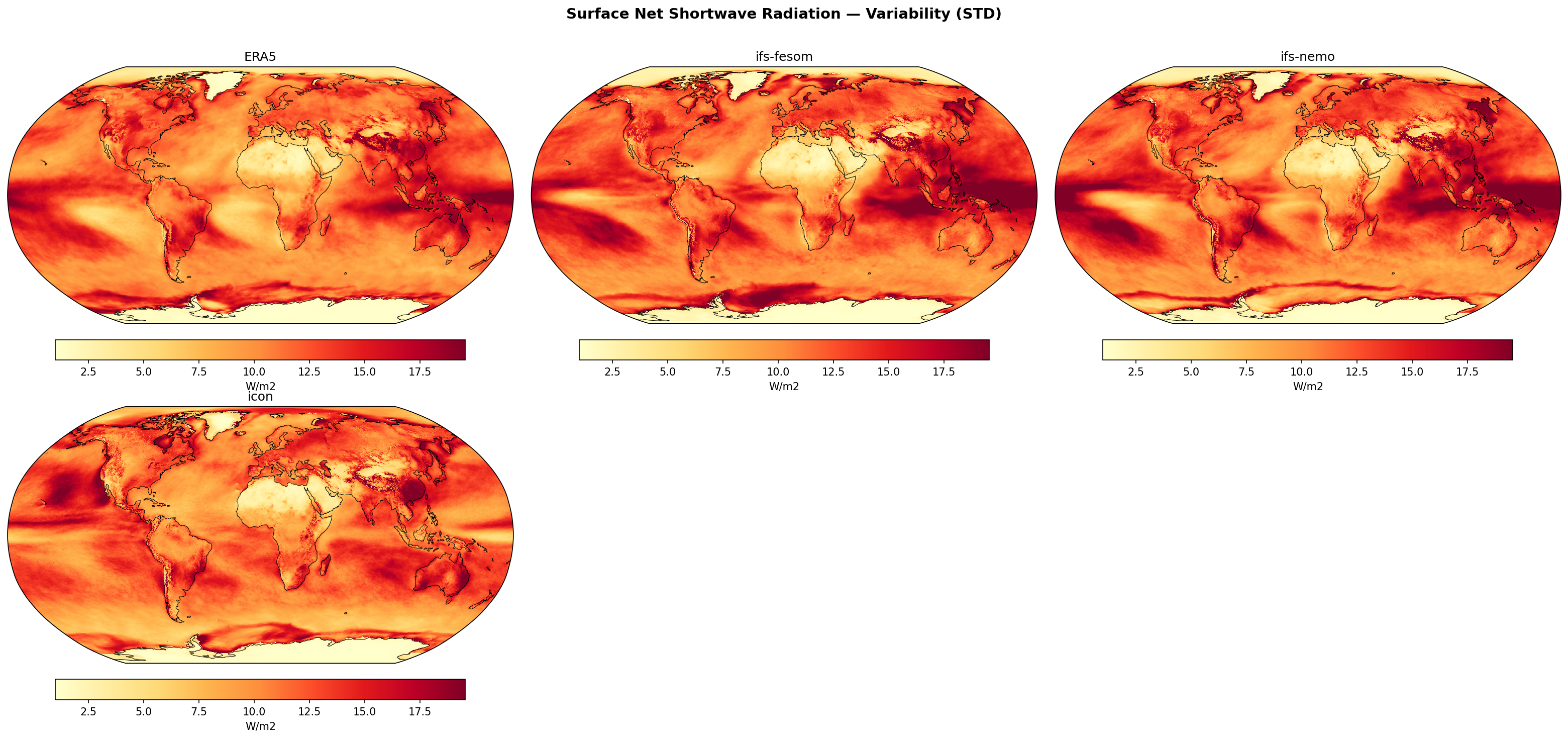
Summary high

This diagnostic shows the standard deviation of deseasonalised surface net shortwave radiation (SSR), serving as a proxy for interannual cloud cover variability. While all models reproduce the major variability centres in the tropics and mid-latitudes, the IFS-based models exhibit higher variability amplitudes than ERA5, particularly in the ENSO region and Southern Ocean.

Key Findings

IFS-FESOM and IFS-NEMO are nearly identical, exhibiting a positive bias in global mean variability (+0.76 to +0.83 W/m²) relative to ERA5.
ICON matches the global mean variability of ERA5 almost perfectly (diff_gmean ~0.01 W/m²) but has the highest spatial RMSE (3.47 W/m²), indicating correct magnitude but displaced spatial patterns.
In the Tropical Pacific, IFS models show a strong, coherent tongue of high variability (>17.5 W/m²) extending westward, indicative of strong ENSO-driven cloud radiative effects, which appears more intense than in ERA5.
IFS models overestimate variability in the Southern Ocean compared to ERA5 and ICON.

Spatial Patterns

The dominant spatial feature is the high variability associated with the El Niño–Southern Oscillation (ENSO) in the central and eastern Tropical Pacific. Secondary maxima occur in the Indian Ocean, the Amazon, and along mid-latitude storm tracks (North Atlantic, Southern Ocean). Low variability characterises the subtropical dry zones and stable ocean gyres. The IFS models display a sharper, more defined variability structure in the Pacific cold tongue region compared to the more diffuse pattern in ICON and ERA5.

Model Agreement

There is very high agreement between IFS-FESOM and IFS-NEMO, confirming that the atmospheric component (IFS) dominates surface radiation variability. Inter-model spread is largest in the Tropical Pacific and Southern Ocean. ICON diverges from the IFS twins by showing lower variability in the Southern Ocean and a less spatially coherent ENSO signature.

Physical Interpretation

Variability in deseasonalised SSR is primarily driven by interannual fluctuations in cloud cover and optical depth. The intense variability in the Tropical Pacific in IFS models suggests a strong coupling between SST anomalies (ENSO) and convective cloud responses. The high variability in the Southern Ocean for IFS likely reflects vigorous storm track activity and associated cloud dynamics. ICON's high RMSE despite good global mean suggests shifts in the location of these convective zones relative to observations.

Caveats

High variability in polar regions may also be influenced by interannual sea ice variations affecting surface albedo, not just cloud cover.
The analysis focuses on variability amplitude, not the phase or timing of events (e.g., ENSO phasing).

Surface Net Shortwave Radiation — Variability Bias (STD diff)

Variables	rss
Models	ifs-fesom, ifs-nemo, icon
Reference Dataset	ERA5
Units	W/m2
Period	1990–2014
ifs-fesom	Std Gmean: 11.87 · Diff Gmean: 0.83 · Rmse: 2.53
ifs-nemo	Std Gmean: 11.80 · Diff Gmean: 0.76 · Rmse: 2.36
icon	Std Gmean: 11.05 · Diff Gmean: 0.01 · Rmse: 3.47

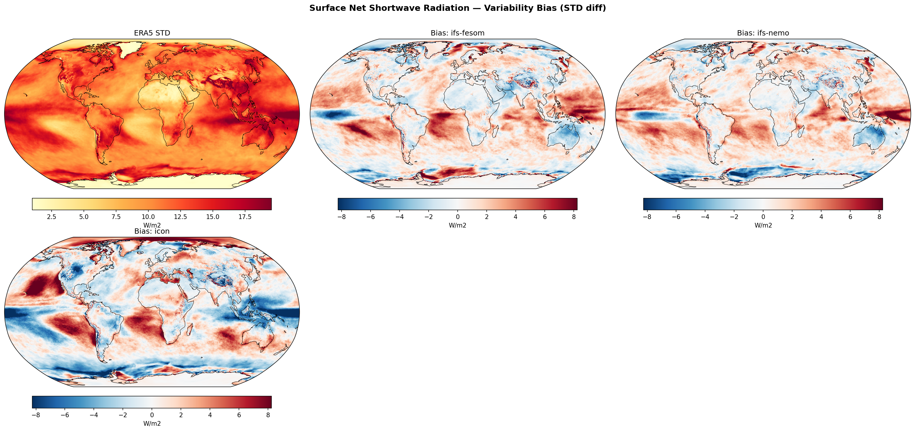
Summary high

This diagnostic evaluates the standard deviation (variability) of surface net shortwave radiation in three high-resolution models compared to ERA5. The IFS-based models generally overestimate variability, particularly in tropical oceans, while ICON exhibits a distinct land-sea contrast with underestimated variability over oceans and overestimated variability over land.

Key Findings

IFS-FESOM and IFS-NEMO show high similarity, with a systematic positive bias in variability (global mean difference ~0.8 W/m²) centered on the tropical ITCZ and trade wind regions.
ICON displays the highest spatial error (RMSE ~3.47 W/m²) despite a near-zero mean bias, driven by a strong dipole: suppressing variability in oceanic storm tracks and the ITCZ (negative bias) while exaggerating it over tropical continents and subtropical stratocumulus regions (positive bias).
A narrow band of underestimated variability along the equatorial Pacific cold tongue is present in the IFS models, contrasting with the overestimated variability in the flanking ITCZ regions.

Spatial Patterns

ERA5 shows peak shortwave variability in the ITCZ and mid-latitude storm tracks. The IFS models exaggerate this variability in the tropical Atlantic, Pacific, and Indian Oceans. In contrast, ICON strongly underestimates variability in the Pacific and Southern Ocean storm tracks and the oceanic ITCZ, but shows intense positive biases over the Amazon, Central Africa, and eastern subtropical ocean basins (stratocumulus decks).

Model Agreement

There is strong agreement between IFS-FESOM and IFS-NEMO, indicating that the atmospheric model physics (IFS) dominate the surface radiation variability signal over the ocean coupling method. ICON diverges significantly from the IFS family, showing opposite bias signs in major climate zones (e.g., negative bias in storm tracks where IFS is mixed/neutral).

Physical Interpretation

Biases are primarily driven by cloud radiative effect variability. The positive bias in IFS suggests convective clouds or trade cumulus are too intermittent or optically variable. ICON's pattern implies overly persistent or stable cloud decks in the oceanic storm tracks (dampening SW variability) and excessively unstable or diurnally active convection over tropical land (amplifying variability). The positive bias in ICON's stratocumulus regions suggests these typically persistent cloud decks break up too frequently in the model.

Caveats

ERA5 is a reanalysis product and relies on its own radiative transfer and cloud parameterisations, which may contain biases compared to direct satellite observations like CERES.
The analysis does not explicitly separate intrinsic cloud variability from variability driven by large-scale dynamics (e.g., shifts in the ITCZ).

Surface Net Shortwave Radiation (Clear-Sky) — Variability (STD)

Variables	rsscs
Models	ifs-fesom, ifs-nemo, icon
Reference Dataset	ERA5
Units	W/m2
Period	1990–2014
ifs-fesom	Std Gmean: 3.99 · Diff Gmean: 0.56 · Rmse: 3.14
ifs-nemo	Std Gmean: 3.65 · Diff Gmean: 0.22 · Rmse: 2.46
icon	Std Gmean: 3.36 · Diff Gmean: -0.07 · Rmse: 3.83

Summary high

This diagnostic shows the standard deviation of deseasonalised surface net shortwave radiation (clear-sky), acting primarily as a proxy for surface albedo variability driven by sea-ice dynamics and snow cover anomalies. All models capture the dominant high-latitude variability patterns seen in ERA5, though with notable differences in magnitude and spatial extent in the polar regions.

Key Findings

High variability (>20 W/m²) is concentrated in the Southern Ocean sea-ice zone and Northern Hemisphere snow/ice margins, corresponding to interannual fluctuations in surface albedo.
IFS-FESOM overestimates variability globally (diff_gmean +0.56 W/m²), particularly exhibiting a broader and more intense band of high variability in the Southern Ocean compared to ERA5.
ICON shows the lowest global mean variability (diff_gmean -0.07 W/m²) but the highest spatial error (RMSE 3.83 W/m²), indicating a mismatch in the precise location of sea-ice/snow variability, particularly in the Southern Ocean.
IFS-NEMO demonstrates the best agreement with ERA5, having the lowest RMSE (2.46 W/m²) and a moderate positive bias (+0.22 W/m²).

Spatial Patterns

Variability is minimal (<5 W/m²) over ice-free oceans and tropical land where albedo is stable. It peaks significantly in the marginal ice zones (Southern Ocean, Barents Sea, Labrador Sea) and over Northern Hemisphere continental snow transition zones (Siberia, Canada), where ephemeral ice/snow cover drives large changes in clear-sky absorption.

Model Agreement

Models agree on the general latitudinal distribution but diverge in the marginal ice zones. IFS-NEMO most closely replicates the ERA5 pattern. IFS-FESOM produces a 'hotter' map with excessive variability in the Antarctic sea-ice belt. ICON's variability band in the Southern Ocean is narrower, and it shows weaker variability over some Northern Hemisphere land regions compared to the IFS variants.

Physical Interpretation

Since cloud effects are removed (clear-sky), variability in surface net shortwave radiation is almost exclusively driven by surface albedo anomalies. Regions of high variability identify where the surface state flips between low-albedo (water/soil) and high-albedo (ice/snow). The excessive variability in IFS-FESOM suggests it may have a more dynamic or variable sea-ice extent/concentration than observed, whereas ICON's sea ice or snow cover appears more stable or spatially constrained.

Caveats

Differences may partly stem from how 'clear-sky' fluxes are computed (e.g., radiative transfer calls) across different model architectures.
ERA5 reanalysis itself relies on modelled albedo and assimilated ice concentration in polar regions, which has uncertainties.

Surface Net Shortwave Radiation (Clear-Sky) — Variability Bias (STD diff)

Variables	rsscs
Models	ifs-fesom, ifs-nemo, icon
Reference Dataset	ERA5
Units	W/m2
Period	1990–2014
ifs-fesom	Std Gmean: 3.99 · Diff Gmean: 0.56 · Rmse: 3.14
ifs-nemo	Std Gmean: 3.65 · Diff Gmean: 0.22 · Rmse: 2.46
icon	Std Gmean: 3.36 · Diff Gmean: -0.07 · Rmse: 3.83

Summary high

This figure evaluates the interannual variability of clear-sky surface net shortwave radiation, acting as a proxy for surface albedo variability driven by sea ice and snow cover dynamics.

Key Findings

ifs-nemo demonstrates the best agreement with ERA5, showing the lowest RMSE (2.46 W/m²) and minimal widespread bias.
ifs-fesom exhibits excessive variability (positive bias >15 W/m²) in dynamic sea ice regions, particularly the East Greenland Current and Weddell Sea.
icon significantly underestimates variability (negative bias) over Northern Hemisphere snow-covered land and the Southern Ocean marginal ice zone.

Spatial Patterns

Biases are strongly polar-amplified, mirroring the regions of maximum variability in the ERA5 reference (sea ice margins and snow lines). Tropical and subtropical oceans show negligible biases (<2 W/m²). Strong dipoles in the Southern Ocean suggest spatial shifts in the marginal ice zone variability.

Model Agreement

The two IFS-based models share a tendency towards positive bias in the Arctic sea ice export regions (East Greenland), though ifs-nemo is dampened compared to ifs-fesom. ICON diverges significantly, showing widespread negative biases (too stable) over Eurasian and North American landmasses where IFS models are closer to neutral.

Physical Interpretation

Since clear-sky net shortwave variability is dominated by surface albedo changes in high latitudes, the biases reflect errors in the interannual stability of the cryosphere. The positive biases in ifs-fesom suggest a too-dynamic sea ice edge or excessive fluctuation in concentration. The negative biases in icon over land suggest snow cover that is either too persistent (saturated albedo) or insufficiently sensitive to interannual climate drivers compared to ERA5.

Caveats

Differences in land surface albedo parameterizations (e.g., vegetation masking of snow) can influence the magnitude of variability.
The analysis assumes 'clear-sky' diagnostics are calculated consistently across models and ERA5.

TOA Net Shortwave Radiation — Variability (STD)

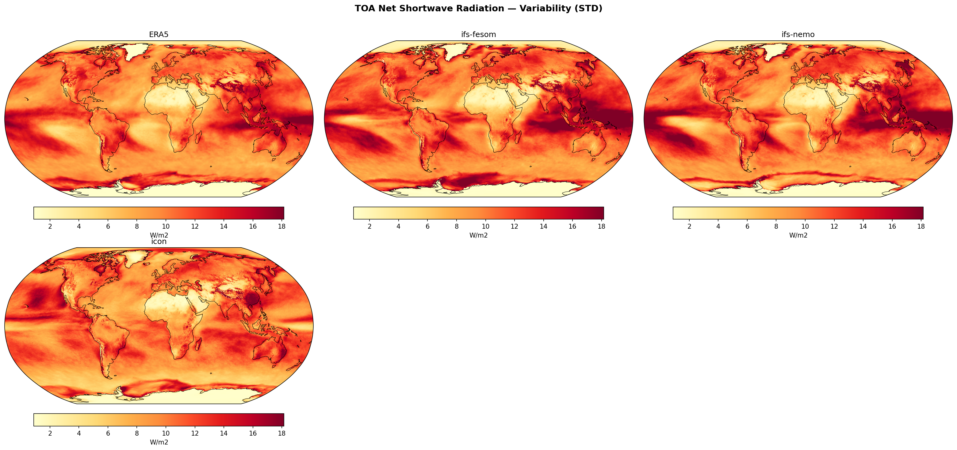
Variables	rst
Models	ifs-fesom, ifs-nemo, icon
Reference Dataset	ERA5
Units	W/m2
Period	1990–2014
ifs-fesom	Std Gmean: 10.80 · Diff Gmean: 0.84 · Rmse: 2.39
ifs-nemo	Std Gmean: 10.71 · Diff Gmean: 0.75 · Rmse: 2.24
icon	Std Gmean: 9.76 · Diff Gmean: -0.20 · Rmse: 3.17

Summary high

This diagnostic compares the standard deviation of deseasonalised and detrended TOA Net Shortwave Radiation (1990–2014), serving as a proxy for cloud cover variability across three high-resolution models and ERA5.

Key Findings

IFS-FESOM and IFS-NEMO exhibit nearly identical spatial patterns and magnitudes, confirming that atmospheric physics dominates shortwave variability regardless of the ocean coupling (FESOM vs NEMO).
Both IFS models overestimate global mean variability (~10.7-10.8 W/m²) compared to ERA5 (implied ~9.96 W/m²), with positive biases of +0.75 to +0.84 W/m².
ICON slightly underestimates global variability (-0.2 W/m² bias) but exhibits the highest spatial error (RMSE 3.17 W/m² vs ~2.3 W/m² for IFS), indicating it captures the total variance well but displaces the spatial features.
IFS models show intense variability in the Indo-Pacific Warm Pool and Tropical Pacific that exceeds ERA5, suggesting stronger convective activity or ENSO amplitude.

Spatial Patterns

Variability hotspots (>16 W/m²) are concentrated in the Tropical Pacific (ENSO signature), Indo-Pacific Warm Pool, and Southern Ocean storm tracks. Low variability (<4 W/m²) characterizes stable subtropical gyres and desert regions. The IFS models display a more coherent and intense ENSO-like tongue in the Pacific compared to ICON.

Model Agreement

High agreement between the two IFS configurations. Moderate agreement between IFS and ERA5 (IFS captures structure but overestimates magnitude). Lower agreement for ICON, which struggles with the spatial distribution of tropical variability relative to ERA5.

Physical Interpretation

Since solar seasonality is removed, variability in Net Shortwave Radiation is driven primarily by cloud cover fluctuations. The patterns map to regions of high convective variance (ITCZ, SPCZ, Warm Pool) and synoptic storm activity (Southern Ocean). The higher variability in IFS suggests more active or sensitive cloud-radiative responses to sea surface temperature anomalies (e.g., ENSO) compared to ICON.

Caveats

ERA5 reanalysis relies on model physics for radiative fluxes and clouds, which may differ from direct satellite observations (CERES).
The 25-year period is sufficient for interannual variability (ENSO) but may not fully capture decadal variability.

TOA Net Shortwave Radiation — Variability Bias (STD diff)

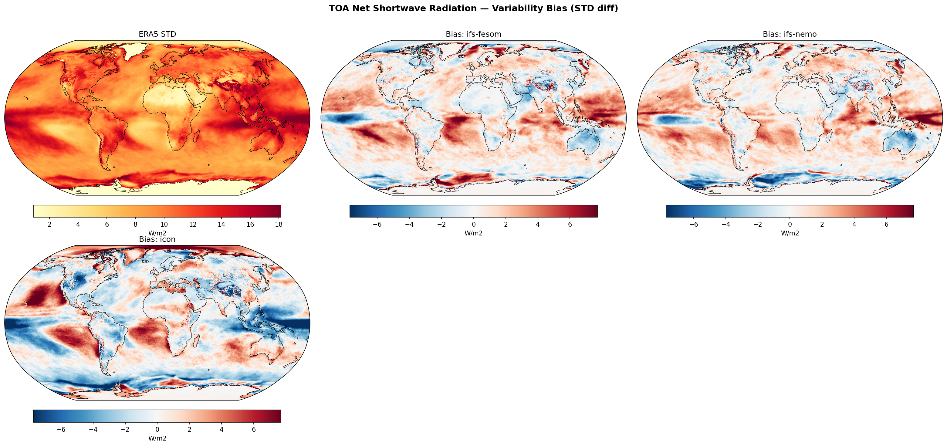
Variables	rst
Models	ifs-fesom, ifs-nemo, icon
Reference Dataset	ERA5
Units	W/m2
Period	1990–2014
ifs-fesom	Std Gmean: 10.80 · Diff Gmean: 0.84 · Rmse: 2.39
ifs-nemo	Std Gmean: 10.71 · Diff Gmean: 0.75 · Rmse: 2.24
icon	Std Gmean: 9.76 · Diff Gmean: -0.20 · Rmse: 3.17

Summary high

This figure evaluates the variability (standard deviation) of TOA Net Shortwave Radiation across three models (ifs-fesom, ifs-nemo, ICON) relative to ERA5 reanalysis for the period 1990–2014.

Key Findings

IFS models (fesom and nemo) exhibit nearly identical bias patterns, characterized by a general overestimation of SW variability (global mean bias ~+0.8 W/m²), particularly in the tropical Atlantic and Eastern Pacific ITCZ.
ICON displays a distinct spatial bias structure with a slight global underestimation (-0.2 W/m²), comprising strong negative biases in the Maritime Continent and storm tracks, contrasted by intense positive biases in the eastern boundary stratocumulus regions (e.g., off Peru and Angola).
A notable dipole exists in the Tropical Pacific for IFS models: variability is underestimated in the central equatorial region (Warm Pool edge) but strongly overestimated in the eastern Pacific.
In the Southern Ocean, IFS models tend to overestimate variability, whereas ICON generally underestimates it.

Spatial Patterns

ERA5 shows peak variability in the ITCZ, SPCZ, and storm tracks. IFS models amplify variability along the tropical rain belts and subtropical highs but dampen it in the central Pacific. ICON shows a 'zonal' bias contrast: suppressed variability in the western Pacific/Indian Ocean (deep convection zones) and excessive variability in the eastern ocean basins (stratocumulus zones).

Model Agreement

High agreement between ifs-fesom and ifs-nemo indicates the atmospheric model dominates SW variability characteristics. Low agreement between IFS and ICON, which show opposite signs of bias in key regions like the Maritime Continent and Southern Ocean.

Physical Interpretation

TOA SW variability is primarily driven by cloud cover fluctuations. Positive biases suggest models produce clouds that are too transient or convective systems that shift position too frequently (e.g., 'flashing' convection). ICON's negative bias in the Maritime Continent suggests overly persistent cloud cover or insufficient convective intermittency. The strong positive bias in stratocumulus regions for ICON suggests difficulties in maintaining stable cloud decks, leading to unrealistic clearing/formation cycles.

Caveats

Reference is ERA5 reanalysis, which relies on its own cloud parameterizations, rather than direct satellite observations like CERES (though patterns likely align).
Analysis does not distinguish between intraseasonal (MJO) and interannual (ENSO) timescales, both of which contribute to the STD.

TOA Net Shortwave Radiation (Clear-Sky) — Variability (STD)

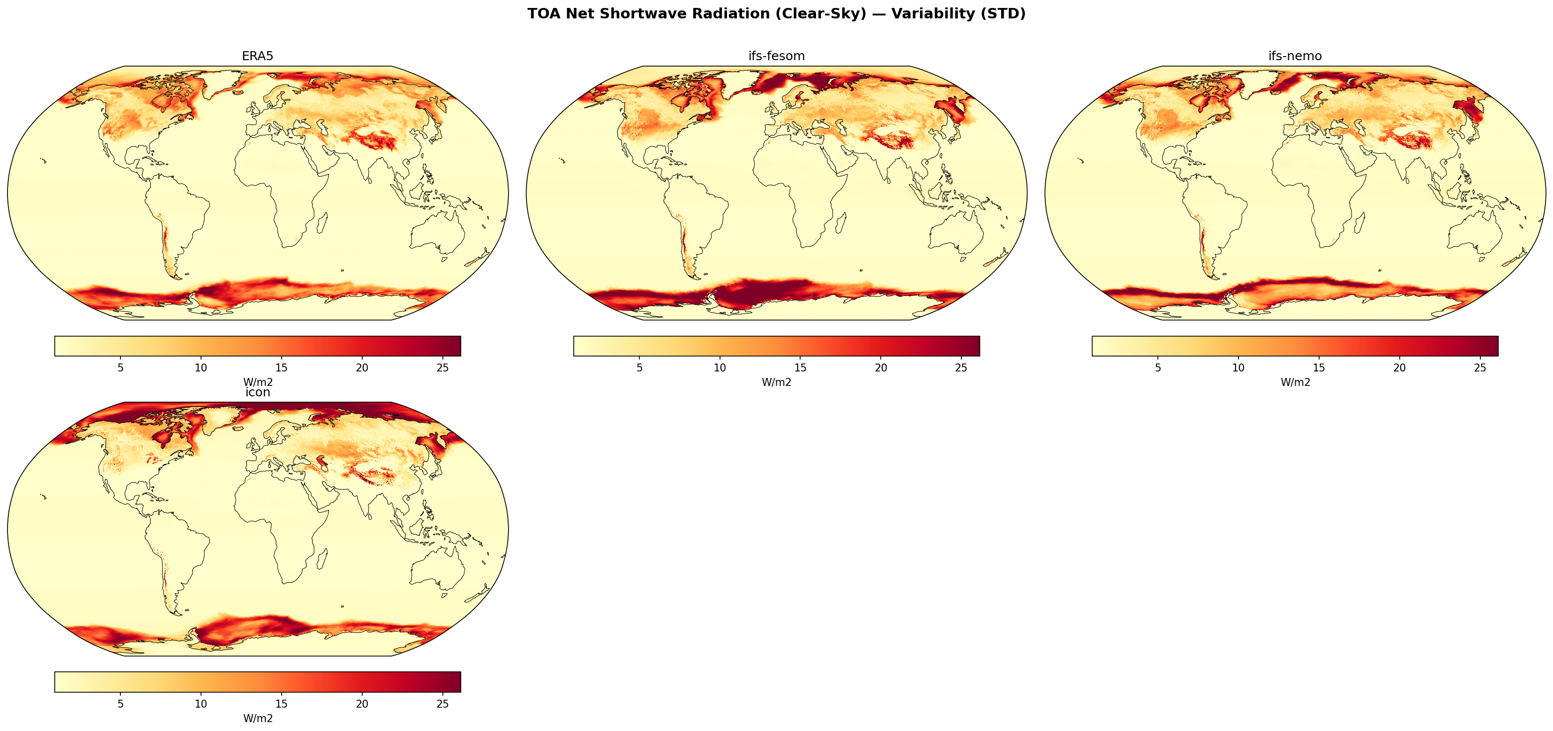
Variables	rstcs
Models	ifs-fesom, ifs-nemo, icon
Reference Dataset	ERA5
Units	W/m2
Period	1990–2014
ifs-fesom	Std Gmean: 3.42 · Diff Gmean: 0.52 · Rmse: 2.97
ifs-nemo	Std Gmean: 3.13 · Diff Gmean: 0.23 · Rmse: 2.30
icon	Std Gmean: 3.06 · Diff Gmean: 0.16 · Rmse: 3.56

Summary high

This diagnostic displays the standard deviation of clear-sky TOA net shortwave radiation, effectively serving as a proxy for the temporal variability of surface albedo (primarily snow and sea ice) over the 1990–2014 period.

Key Findings

Variability is almost exclusively confined to high-latitude cryospheric regions (sea ice margins and snow-covered land), with negligible variability over open oceans, confirming the dominant role of surface albedo in clear-sky SW fluctuations.
ifs-fesom exhibits a marked overestimation of variability in the Southern Hemisphere sea ice zone, suggesting excessive interannual or month-to-month fluctuations in sea ice extent compared to ERA5.
ifs-nemo performs best spatially (lowest RMSE of 2.30 W/m²), capturing the ERA5 patterns more closely than ifs-fesom, though still showing elevated variability in the Antarctic sea ice belt.
icon has the lowest global mean bias (+0.16 W/m²) but the highest spatial error (RMSE 3.56 W/m²), indicating that while the total magnitude of variability is accurate, its spatial distribution is misplaced, particularly visible in the high Arctic.

Spatial Patterns

High variability (>15-20 W/m²) coincides with the marginal sea ice zones (Southern Ocean, Sea of Okhotsk, Hudson Bay) and continental regions with variable snow cover (Eurasia, North America). The Southern Ocean variability band is notably broader and more intense in the ifs-fesom simulation than in ERA5.

Model Agreement

All models agree on the location of variability hotspots but differ significantly in amplitude. The IFS-based models (ifs-fesom, ifs-nemo) systematically overestimate variability in the Southern Ocean compared to ERA5. ICON shows distinct discrepancies in the Arctic, with intense variability near the pole not seen as strongly in the other datasets.

Physical Interpretation

In the absence of clouds (clear-sky), fluctuations in Net TOA Shortwave radiation are driven almost entirely by surface albedo changes. The patterns therefore reveal where models have unstable or highly variable snow and sea ice cover. The excessive variability in the Southern Ocean for IFS models likely reflects a highly dynamic sea ice edge or large fluctuations in concentration.

Caveats

Clear-sky fluxes are diagnostic quantities; differences in how 'clear-sky' is defined or sampled between the models and the ERA5 reanalysis could contribute to minor discrepancies.
The analysis does not distinguish between interannual variability and seasonal cycle residuals, though the data is described as deseasonalised.

TOA Net Shortwave Radiation (Clear-Sky) — Variability Bias (STD diff)

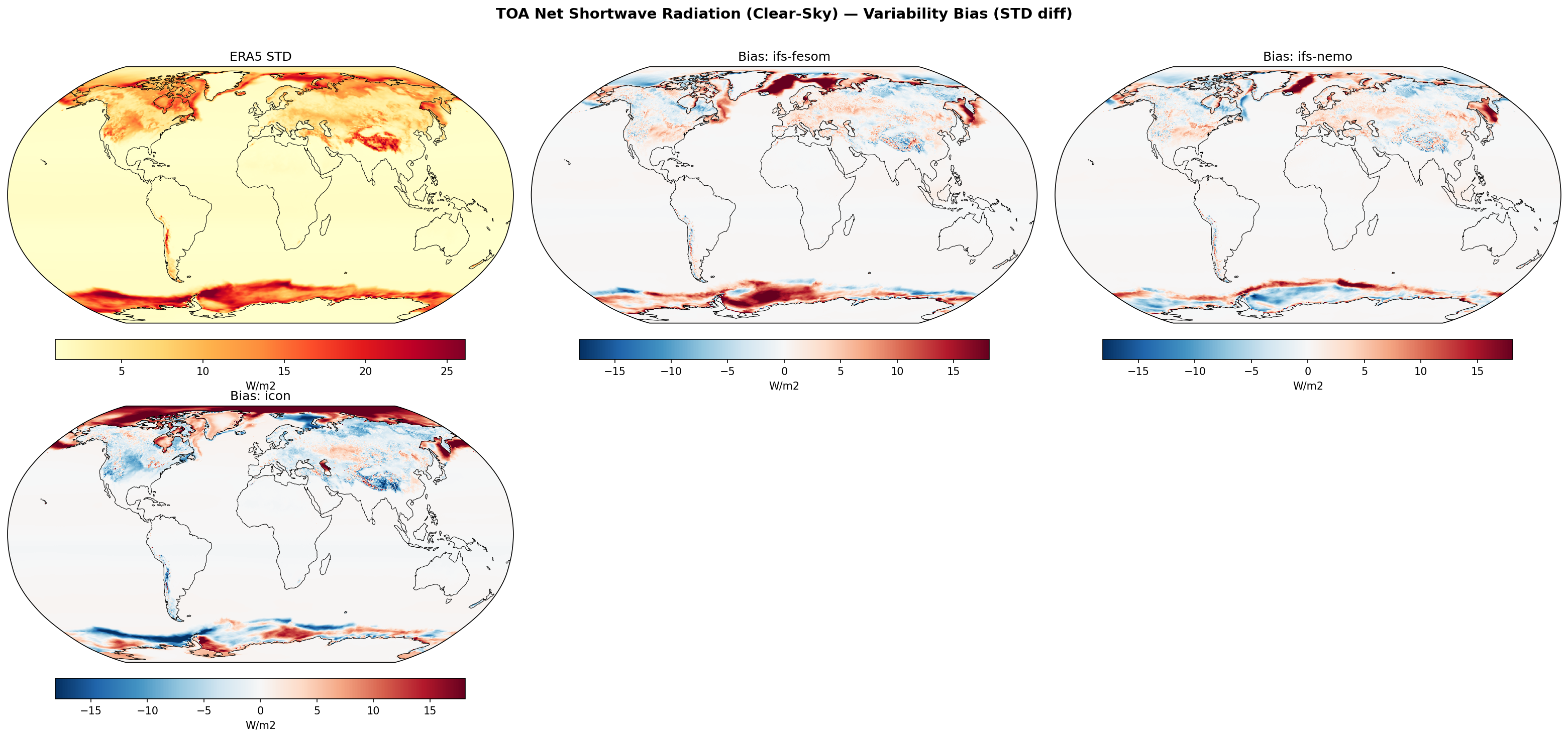
Variables	rstcs
Models	ifs-fesom, ifs-nemo, icon
Reference Dataset	ERA5
Units	W/m2
Period	1990–2014
ifs-fesom	Std Gmean: 3.42 · Diff Gmean: 0.52 · Rmse: 2.97
ifs-nemo	Std Gmean: 3.13 · Diff Gmean: 0.23 · Rmse: 2.30
icon	Std Gmean: 3.06 · Diff Gmean: 0.16 · Rmse: 3.56

Summary high

This diagnostic evaluates the variability (standard deviation) of clear-sky TOA Net Shortwave Radiation, primarily serving as a proxy for surface albedo variability driven by sea ice and snow cover dynamics.

Key Findings

Variability in clear-sky shortwave radiation is dominated by high-latitude cryospheric regions (sea ice margins and seasonal snow cover), where surface albedo changes significantly.
IFS-NEMO demonstrates the best agreement with ERA5 (RMSE ~2.30 W/m²), showing smaller biases than the other models.
Both IFS models (FESOM and NEMO) exhibit positive variability biases (excessive fluctuation) in the North Atlantic marginal ice zones (Labrador and Greenland Seas) and parts of the Southern Ocean.
ICON shows the largest discrepancies (RMSE ~3.56 W/m²), characterised by a distinct underestimation of variability (negative bias) over the central Arctic, Antarctic coastal zones, and Northern Hemisphere snow-covered land.

Spatial Patterns

ERA5 shows peak variability (>25 W/m²) over the Southern Ocean sea ice zone and Northern Hemisphere snow transition regions. Model biases are spatially coherent: IFS models show strong positive biases (excess variability) in the Labrador Sea, Greenland Sea, and Weddell Sea. ICON displays a contrasting pattern with widespread negative biases (insufficient variability) over the polar caps and NH continents, but strong positive biases in the Bering Sea and North Atlantic sub-polar gyre.

Model Agreement

IFS-NEMO and IFS-FESOM share similar bias structures (dipoles along ice edges), though IFS-FESOM has larger magnitudes. ICON diverges significantly, often showing biases of opposite sign (e.g., negative bias in the Arctic where IFS is neutral or positive) and the highest spatial RMSE.

Physical Interpretation

Since clouds are removed, variability in Net SW TOA is driven by surface albedo anomalies. The observed biases indicate mismatches in the interannual variability of sea ice extent and snow cover. The positive biases in IFS models suggest a too-dynamic sea ice edge or excessive formation/melting cycles in marginal zones. ICON's negative biases over land and polar caps suggest snow and ice cover are too temporally stable or lack the observed sensitivity to interannual forcing.

Caveats

Differences in the definition or sampling of 'clear-sky' conditions between the models and ERA5 reanalysis could contribute to residual biases, though the albedo signal dominates.
The analysis does not distinguish between sea ice concentration variability and thickness-driven albedo changes, though concentration is the primary SW driver.

2m Temperature — Variability (STD)

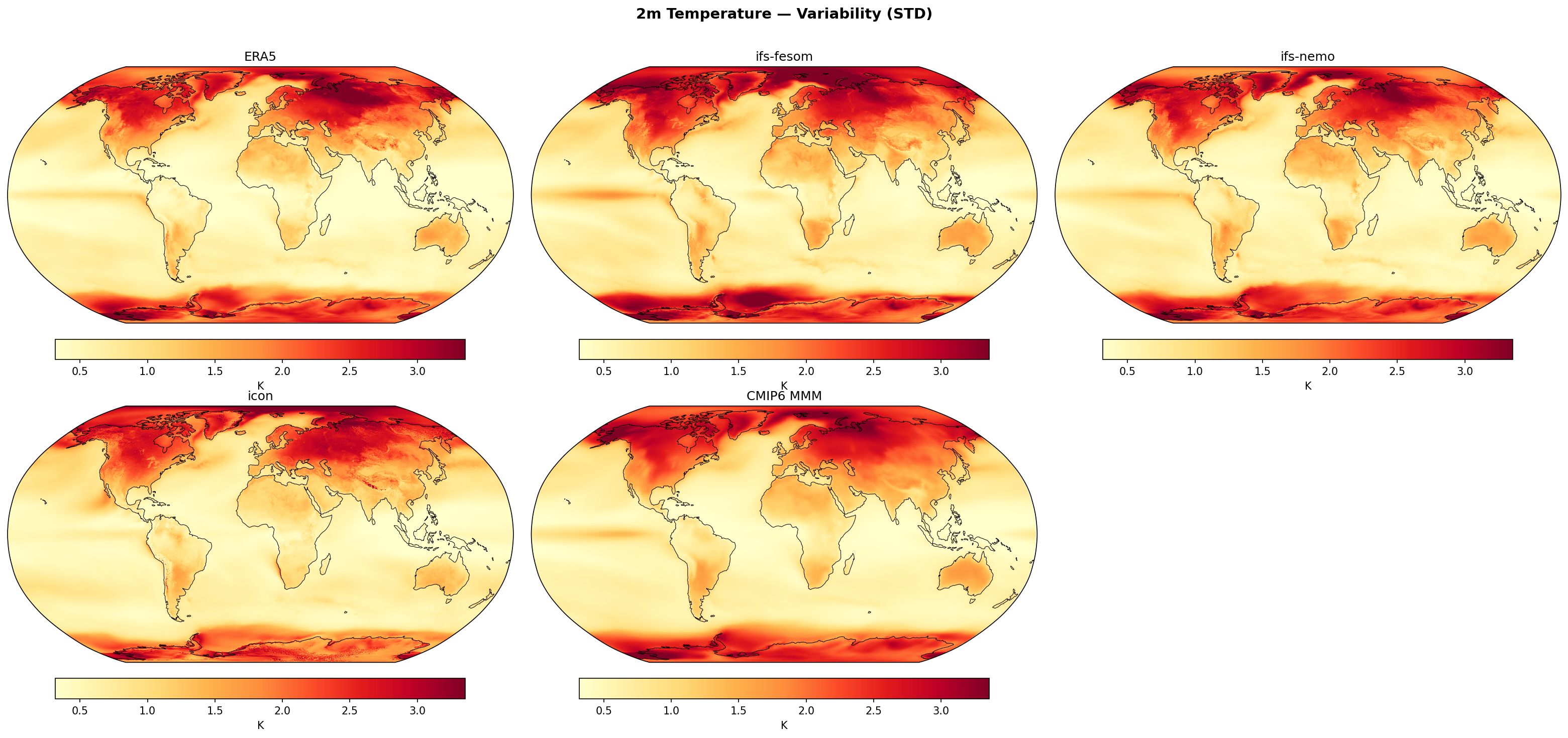
Variables	tas
Models	ifs-fesom, ifs-nemo, icon, CMIP6 MMM
Reference Dataset	ERA5
Units	K
Period	1990–2014
ifs-fesom	Std Gmean: 1.10 · Diff Gmean: 0.14 · Rmse: 0.28
ifs-nemo	Std Gmean: 1.02 · Diff Gmean: 0.07 · Rmse: 0.18
icon	Std Gmean: 0.99 · Diff Gmean: 0.04 · Rmse: 0.25
CMIP6 MMM	Std Gmean: 1.04 · Diff Gmean: 0.08 · Rmse: 0.18

Summary high

This figure compares the standard deviation of deseasonalised, detrended monthly 2m temperature anomalies (1990–2014) across three high-resolution models and the CMIP6 multi-model mean against ERA5 reanalysis. While all models capture the fundamental land-sea contrast and ENSO variability, significant differences appear in the Southern Ocean sea ice zones.

Key Findings

All models successfully reproduce the primary variability pattern: high variability (>3 K) over high-latitude continents (Siberia, N. America) and low variability (<1 K) over tropical oceans.
ifs-fesom exhibits a large region of excessive variability in the Weddell Sea (Southern Ocean), driving the highest global RMSE (0.28 K) and mean bias (+0.14 K).
ifs-nemo shows the best agreement with ERA5 among the individual models (RMSE ~0.18 K), accurately capturing the magnitude and spatial distribution of variability in the marginal ice zones.
icon captures the global mean variability well (lowest mean bias +0.036 K) but has a higher spatial RMSE (0.25 K) than ifs-nemo, with somewhat noisy patterns along the Antarctic coast.

Spatial Patterns

Variability is dominated by the thermal inertia contrast between land and ocean. Maxima occur over NH continents. Localised maxima exist in the Tropical Pacific (ENSO tongue) and along sea-ice edges (marginal ice zones). The Weddell Sea anomaly in ifs-fesom is a distinct outlier feature not present in ERA5.

Model Agreement

ifs-nemo aligns closely with ERA5 and the CMIP6 MMM, particularly in the Southern Hemisphere. ifs-fesom diverges significantly in the Southern Ocean. icon generally agrees with observations but shows grainier artifacts in polar regions compared to the smoother ERA5 fields.

Physical Interpretation

High continental variability results from the low heat capacity of land responding to synoptic and seasonal forcing. The bands of high variability around sea-ice edges (Antarctic, Arctic) represent the intermittency of sea-ice cover (insulating) versus open water (exposed). The excessive variability in ifs-fesom's Weddell Sea is likely a signature of frequent open-ocean deep convection events (polynyas) or unstable sea-ice extent in that model configuration.

Caveats

The CMIP6 MMM is naturally smoother than individual realizations due to averaging out internal variability.
High variability in model sea-ice zones may stem from displacement of the ice edge rather than true temperature variance errors.

2m Temperature — Variability Bias (STD diff)

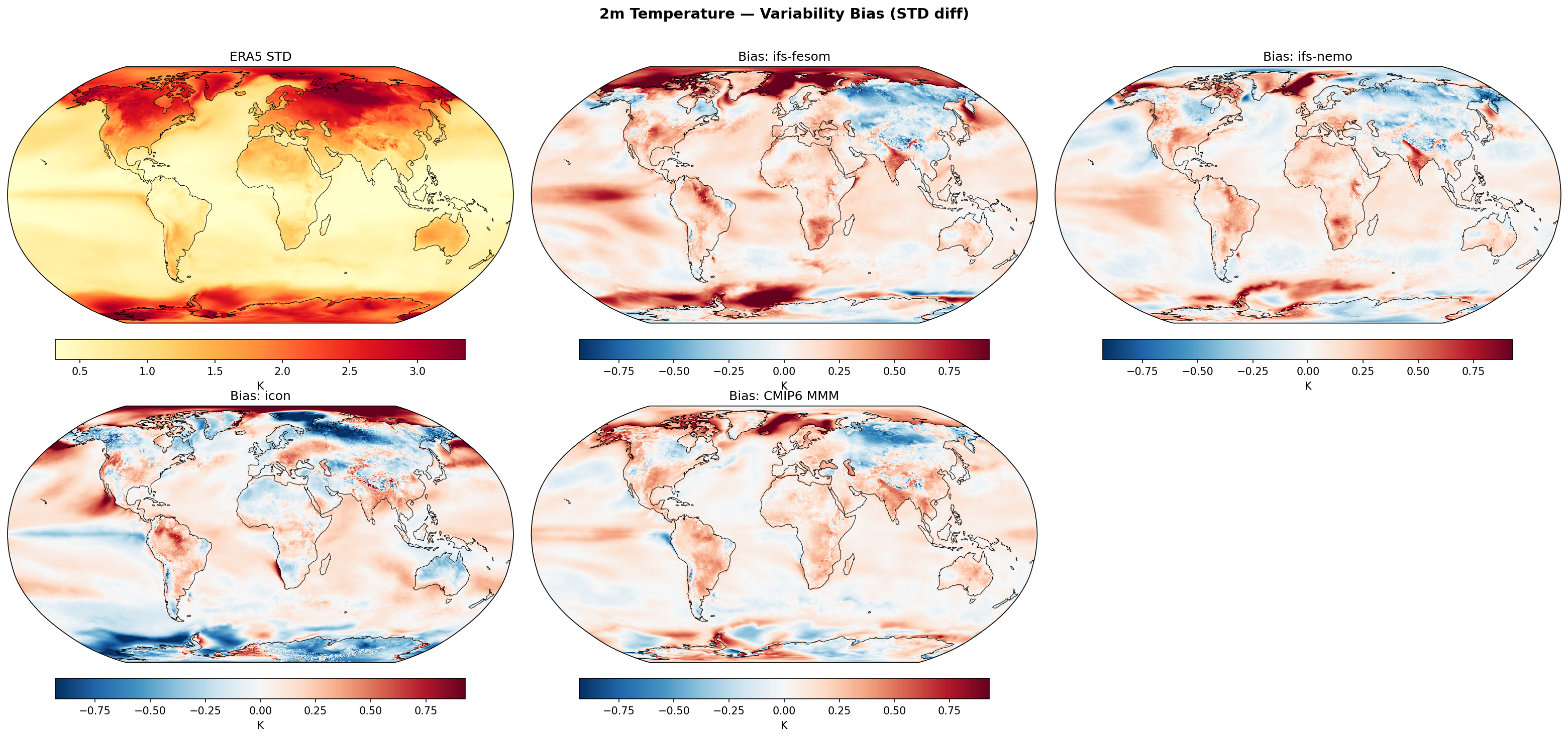
Variables	tas
Models	ifs-fesom, ifs-nemo, icon, CMIP6 MMM
Reference Dataset	ERA5
Units	K
Period	1990–2014
ifs-fesom	Std Gmean: 1.10 · Diff Gmean: 0.14 · Rmse: 0.28
ifs-nemo	Std Gmean: 1.02 · Diff Gmean: 0.07 · Rmse: 0.18
icon	Std Gmean: 0.99 · Diff Gmean: 0.04 · Rmse: 0.25
CMIP6 MMM	Std Gmean: 1.04 · Diff Gmean: 0.08 · Rmse: 0.18

Summary high

This figure evaluates the variability (standard deviation) of 2m temperature in three high-resolution models and the CMIP6 multi-model mean against ERA5 reanalysis for the period 1990–2014. Generally, the models tend to overestimate temperature variability, particularly in the tropical Pacific and high latitudes, with distinct regional bias patterns separating the model formulations.

Key Findings

All models exhibit a positive variability bias in the tropical Pacific, indicative of excessive ENSO amplitude relative to the 1990–2014 observed period.
ifs-nemo shows the best overall agreement with ERA5 (RMSE = 0.18 K), closely matching the CMIP6 multi-model mean performance, whereas ifs-fesom has the largest global overestimation (diff_gmean = +0.14 K).
ifs-fesom displays strong positive variability biases in the Arctic and Antarctic regions, suggesting excessive fluctuations in sea ice extent or surface fluxes compared to ifs-nemo.
icon presents a unique bias structure with strong positive variability over tropical land masses (Amazon, Central Africa) and negative variability biases in the high-latitude Southern Ocean and North Atlantic.

Spatial Patterns

The dominant spatial feature is the 'bullseye' of positive bias in the central-to-eastern equatorial Pacific, present in all models but strongest in ifs-fesom. Over land, icon stands out with intense positive biases in the Amazon and Congo basins, contrasting with the more neutral land biases in the IFS models. In the polar regions, ifs-fesom is uniformly 'hot' (too variable), while icon shows regions of suppressed variability (blue) around the Antarctic coast.

Model Agreement

ifs-nemo and the CMIP6 MMM show the highest agreement with observations, sharing similar RMSE values (~0.18 K). ifs-fesom and icon diverge significantly: ifs-fesom is systematically too variable globally (red dominance), while icon has large compensating errors (high RMSE of 0.25 K despite a low global mean difference of +0.04 K) due to contrasting land (positive) and high-latitude ocean (negative) biases.

Physical Interpretation

The tropical Pacific bias suggests that the coupled models may have an overly active Bjerknes feedback or are capturing a canonical ENSO amplitude that exceeds the specific variability observed during the 1990–2014 window. The high variability in ifs-fesom's polar regions likely points to instability in the marginal sea ice zone (excessive freeze/melt cycles or advection). In contrast, icon's excessive land variability implies issues with land-atmosphere coupling, possibly related to soil moisture drying out too quickly, shifting the energy balance towards sensible heat and amplifying temperature extremes.

Caveats

The analysis period (1990–2014) is relatively short (25 years) for robustly characterizing low-frequency internal variability modes like ENSO or PDO.
Discrepancies in the tropical Pacific may partly reflect the specific phase of internal variability in the real world (e.g., the prevalence of La Niña-like conditions in the early 2000s) versus the models' free-running internal states.

10m U Wind — Variability (STD)

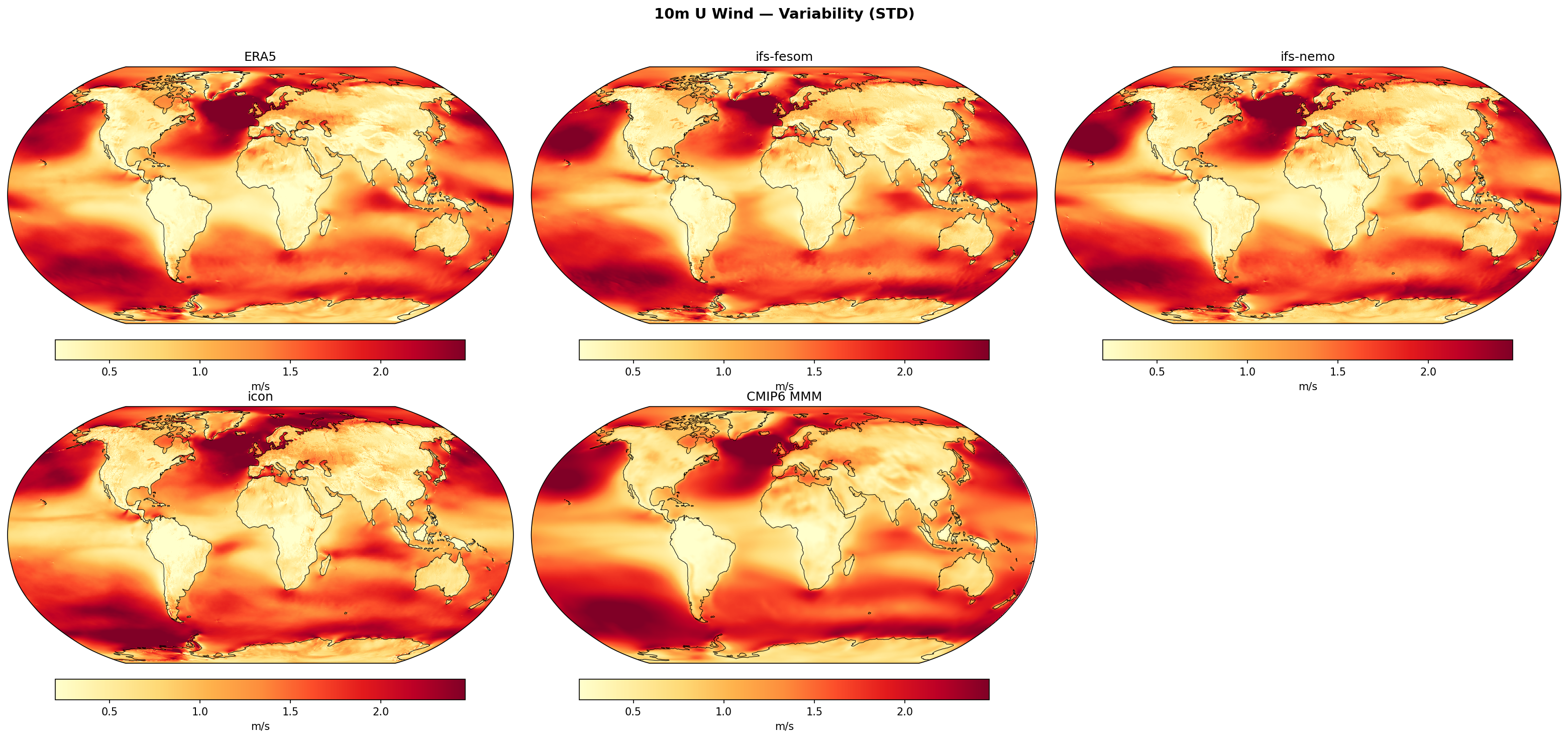
Variables	uas
Models	ifs-fesom, ifs-nemo, icon, CMIP6 MMM
Reference Dataset	ERA5
Units	m/s
Period	1990–2014
ifs-fesom	Std Gmean: 1.20 · Diff Gmean: 0.02 · Rmse: 0.17
ifs-nemo	Std Gmean: 1.20 · Diff Gmean: 0.02 · Rmse: 0.14
icon	Std Gmean: 1.20 · Diff Gmean: 0.03 · Rmse: 0.27
CMIP6 MMM	Std Gmean: 1.26 · Diff Gmean: 0.09 · Rmse: 0.19

Summary high

This figure evaluates the variability (standard deviation) of deseasonalised monthly 10m zonal wind (U-component), serving as a proxy for storm track activity and low-frequency circulation variability. The high-resolution DestinE models (ifs-fesom, ifs-nemo, icon) capture the spatial structure of global wind variability with high fidelity, with the IFS-based models outperforming the CMIP6 Multi-Model Mean in terms of RMSE.

Key Findings

High-resolution models accurately reproduce the major mid-latitude storm tracks (North Atlantic, North Pacific, Southern Ocean) as bands of high wind variability (>2 m/s).
ifs-nemo achieves the lowest RMSE (0.14 m/s) relative to ERA5, followed by ifs-fesom (0.17 m/s), indicating excellent skill in capturing the amplitude of surface wind fluctuations.
The CMIP6 MMM generally overestimates global mean variability (+0.08 m/s) more than the DestinE models (+0.02 m/s), suggesting high-resolution simulations better constrain the energy of surface wind anomalies.
ICON displays the highest RMSE (0.27 m/s) among all groups (including CMIP6), despite a low global mean bias, suggesting larger regional discrepancies in variability patterns.

Spatial Patterns

Variability is dominated by the mid-latitude westerlies, with distinct maxima in the North Atlantic and North Pacific storm tracks and a continuous high-variability belt in the Southern Ocean (40°S–60°S). Land areas consistently show lower variability (<1.0 m/s) due to surface friction. The Northern Hemisphere tracks exhibit a characteristic SW-NE tilt which is well-captured by all models.

Model Agreement

There is strong structural agreement between ERA5 and all models regarding the placement of high-variability zones. ifs-fesom and ifs-nemo are visually nearly identical to ERA5. ICON captures the main features but statistically deviates more (highest RMSE), possibly due to noise or excessive variability in specific regions like the polar oceans or tropics that is less apparent in the global map view compared to difference plots.

Physical Interpretation

The spatial patterns reflect the dominant influence of synoptic-scale cyclone activity (storm tracks) on monthly wind variance. The high resolution of the DestinE models allows for better representation of sharp gradients in these tracks and topographic steering effects compared to the coarser CMIP6 ensemble. The lower variability over land is a direct result of higher aerodynamic roughness lengths damping surface wind speeds.

Caveats

The analysis uses monthly data, meaning it captures inter-annual and low-frequency sub-seasonal variability rather than high-frequency daily storminess, though the two are physically linked.
The source of ICON's higher RMSE is not immediately spatially distinct in the side-by-side maps and would require a difference map to diagnose (e.g., potential noise at sea-ice edges or orographic drag differences).

10m U Wind — Variability Bias (STD diff)

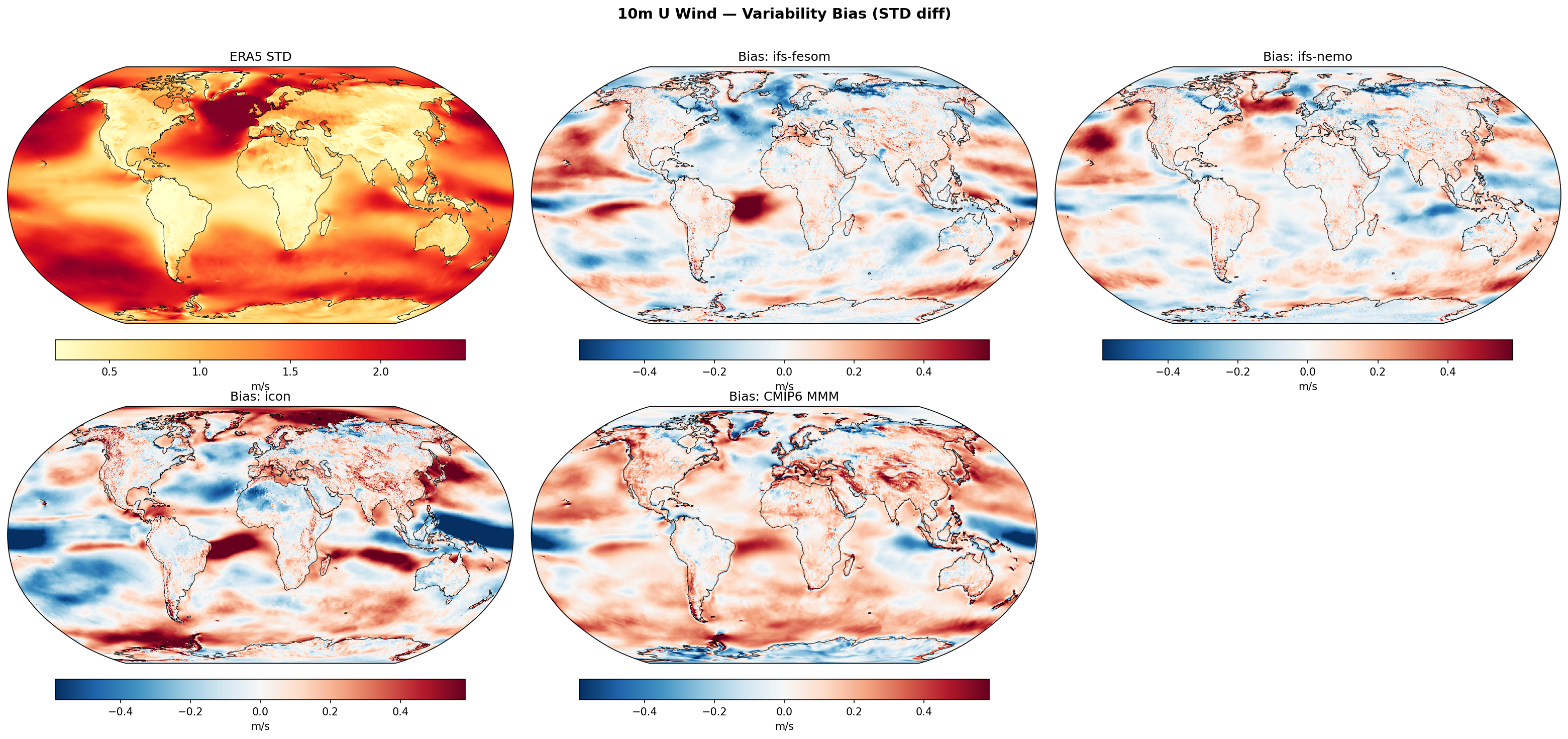
Variables	uas
Models	ifs-fesom, ifs-nemo, icon, CMIP6 MMM
Reference Dataset	ERA5
Units	m/s
Period	1990–2014
ifs-fesom	Std Gmean: 1.20 · Diff Gmean: 0.02 · Rmse: 0.17
ifs-nemo	Std Gmean: 1.20 · Diff Gmean: 0.02 · Rmse: 0.14
icon	Std Gmean: 1.20 · Diff Gmean: 0.03 · Rmse: 0.27
CMIP6 MMM	Std Gmean: 1.26 · Diff Gmean: 0.09 · Rmse: 0.19

Summary high

This diagnostic assesses the variability (standard deviation) of 10m zonal wind (U-wind) in three high-resolution DestinE models and the CMIP6 multi-model mean against ERA5 reanalysis for the period 1990–2014.

Key Findings

ifs-nemo demonstrates the highest skill, with the lowest RMSE (0.14 m/s) and a spatial bias pattern that is largely neutral compared to other models.
icon exhibits a distinct zonal bias contrast: it strongly overestimates variability in the extratropical storm tracks (Southern Ocean, North Atlantic) while underestimating variability in the tropical Indo-Pacific.
ifs-fesom shares the atmospheric core with ifs-nemo but shows larger biases, including underestimation in the North Atlantic storm track and a localized region of excessive variability in the South Atlantic.
The CMIP6 multi-model mean systematically overestimates surface wind variability globally (mean bias +0.09 m/s), whereas the high-resolution models show smaller global mean biases (~0.02 m/s).

Spatial Patterns

ERA5 shows peak variability in the mid-latitude storm tracks (Southern Ocean, North Atlantic, North Pacific). icon exaggerates this meridional gradient, intensifying the storm tracks (red bias) and dampening the tropics (blue bias). ifs-fesom shows a notable dipole in the Atlantic (blue North, red South). All models show higher variability over major mountain ranges (Himalayas, Andes), most pronounced in icon.

Model Agreement

ifs-nemo shows excellent agreement with ERA5. Inter-model divergence is significant: icon and ifs-fesom show opposite biases in the North Atlantic storm track (icon too variable, ifs-fesom too quiet). The CMIP6 ensemble mean is spatially smoother but positively biased over most oceans.

Physical Interpretation

Surface wind variability is primarily driven by synoptic-scale eddies in the extratropics and convective/trade-wind fluctuations in the tropics. The strong positive bias in icon's storm tracks suggests overly energetic synoptic activity or insufficient surface drag. Conversely, icon's tropical dampening implies suppressed variability in trade winds or convective momentum transport. The divergence between ifs-fesom and ifs-nemo (which share an atmospheric model) highlights how different ocean couplings (SST gradients and temporal variance) modulate surface wind variability.

Caveats

ERA5 is a reanalysis product and relies on its own model physics (IFS-based), which may favor the IFS-based models (nemo/fesom) over ICON.
High variability biases over topography in ICON may result from resolution differences or orographic drag parameterization specifics.

10m V Wind — Variability (STD)

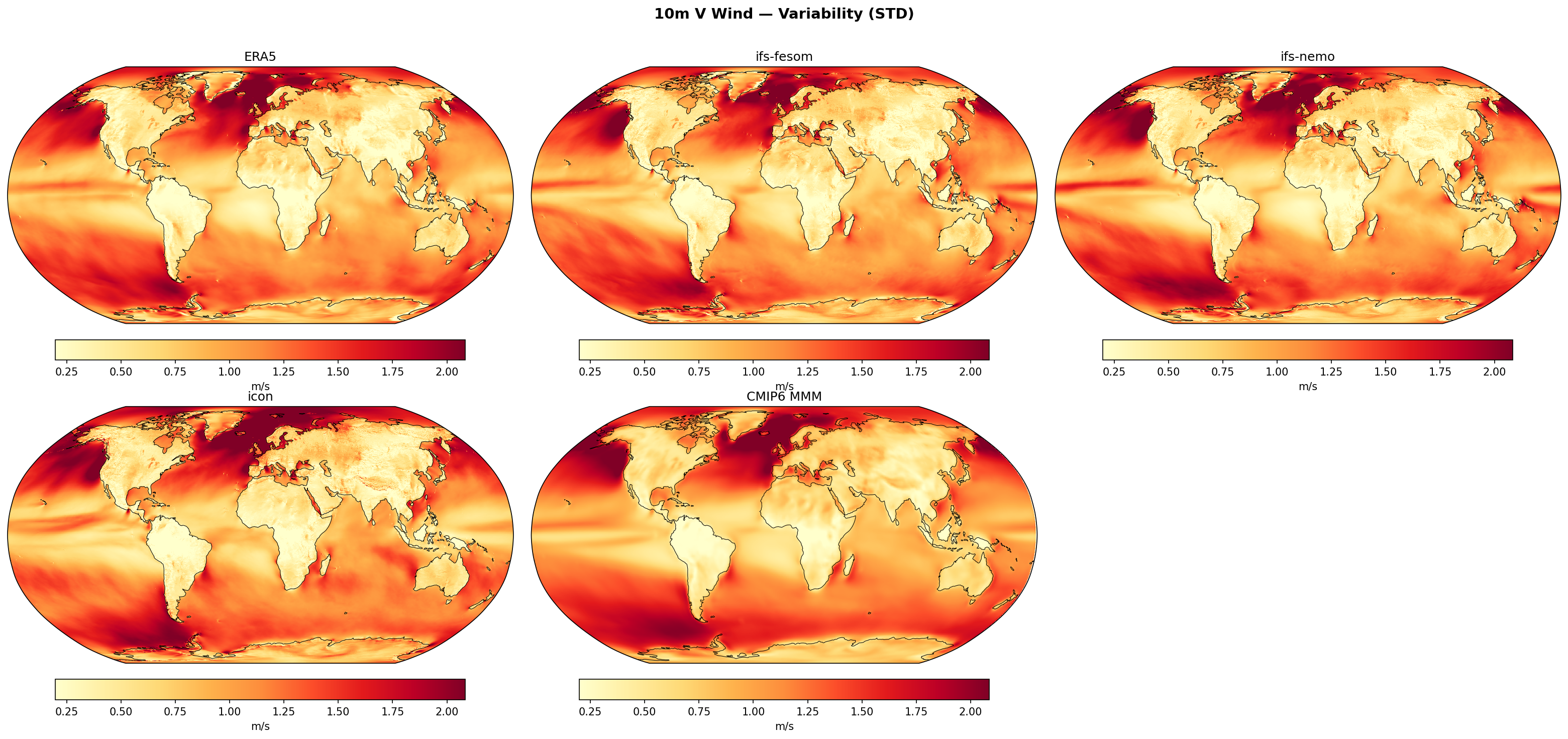
Variables	vas
Models	ifs-fesom, ifs-nemo, icon, CMIP6 MMM
Reference Dataset	ERA5
Units	m/s
Period	1990–2014
ifs-fesom	Std Gmean: 0.94 · Diff Gmean: 0.01 · Rmse: 0.13
ifs-nemo	Std Gmean: 0.95 · Diff Gmean: 0.03 · Rmse: 0.13
icon	Std Gmean: 0.98 · Diff Gmean: 0.05 · Rmse: 0.19
CMIP6 MMM	Std Gmean: 1.00 · Diff Gmean: 0.07 · Rmse: 0.15

Summary high

This diagnostic compares the interannual variability (standard deviation) of 10m meridional wind across three high-resolution models and the CMIP6 multi-model mean against ERA5 reanalysis. The high-resolution models, particularly the IFS variants, reproduce the spatial distribution of wind variability with high skill, capturing key storm track and tropical features.

Key Findings

All models correctly identify the North Atlantic, North Pacific, and Southern Ocean storm tracks as the dominant regions of meridional wind variability (>1.5 m/s).
IFS-NEMO and IFS-FESOM demonstrate the best agreement with ERA5, with RMSE values of ~0.127 m/s and ~0.131 m/s respectively, outperforming both ICON (0.187 m/s) and the CMIP6 MMM (0.152 m/s).
ICON and CMIP6 MMM systematically overestimate global variability (biases of +0.049 m/s and +0.072 m/s), while IFS-FESOM shows the smallest global mean bias (+0.013 m/s).

Spatial Patterns

The maps highlight three main zones of high variability: the extratropical storm tracks in both hemispheres (driven by synoptic eddy activity) and a zonal band in the tropical Pacific associated with the ITCZ and ENSO dynamics. Continents exhibit markedly lower meridional wind variability than oceans. The spatial structure of the Tropical Pacific variability is well-captured by all high-res models.

Model Agreement

There is strong agreement between the two IFS-based models (FESOM and NEMO), reflecting their shared atmospheric component. ICON produces spatially broader and more intense variability features, contributing to its higher RMSE. The CMIP6 MMM captures the large-scale patterns but with smoothed gradients and a higher average magnitude than ERA5.

Physical Interpretation

Meridional wind variability at the surface is a proxy for synoptic-scale activity (cyclone/anticyclone passage) in the mid-latitudes and convergence zone migration in the tropics. The positive bias in variability across models suggests they may be slightly more energetic or have less surface drag dampening than the ERA5 reanalysis. The localized high variability in storm tracks is better resolved in the km-scale simulations compared to the coarser CMIP6 ensemble.

Caveats

The CMIP6 MMM appears smoother due to ensemble averaging, which naturally dampens internal variability relative to single realizations; however, its global mean variability remains notably high.
Comparisons are based on 1990-2014 climatologies; internal multidecadal variability might influence localized discrepancies.

10m V Wind — Variability Bias (STD diff)

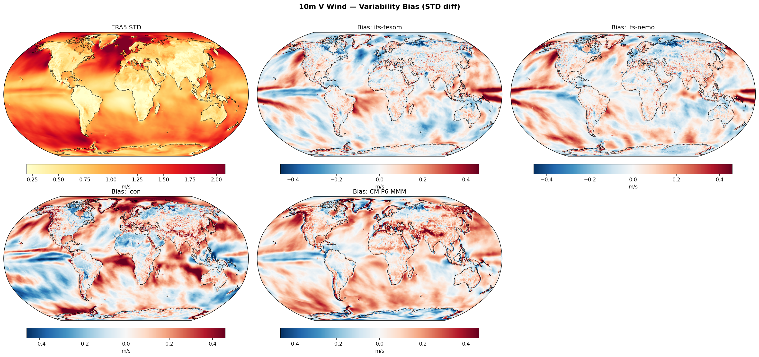
Variables	vas
Models	ifs-fesom, ifs-nemo, icon, CMIP6 MMM
Reference Dataset	ERA5
Units	m/s
Period	1990–2014
ifs-fesom	Std Gmean: 0.94 · Diff Gmean: 0.01 · Rmse: 0.13
ifs-nemo	Std Gmean: 0.95 · Diff Gmean: 0.03 · Rmse: 0.13
icon	Std Gmean: 0.98 · Diff Gmean: 0.05 · Rmse: 0.19
CMIP6 MMM	Std Gmean: 1.00 · Diff Gmean: 0.07 · Rmse: 0.15

Summary high

The figure evaluates the variability of 10m meridional (V) wind, showing that the IFS-based models exhibit similar bias patterns with excess tropical variability, while ICON presents distinct behaviors including strong orographic signatures and suppressed variability in the central Pacific.

Key Findings

IFS-fesom and IFS-nemo show high pattern correlation, characterized by overestimated variability along the tropical convergence zones (ITCZ/SPCZ) and slight underestimation in the Southern Ocean storm track.
ICON displays unique biases: strong high-frequency errors over major mountain ranges (Andes, Himalayas), a notable underestimation of variability in the central Pacific ITCZ (contrasting with IFS), and overestimation in the North Atlantic storm track.
The CMIP6 Multi-Model Mean generally overestimates meridional wind variability globally (diff_gmean +0.07 m/s), particularly over Northern Hemisphere land, whereas the high-resolution DestinE models show smaller global mean biases (+0.01 to +0.05 m/s).
IFS-nemo performs slightly better than IFS-fesom in terms of RMSE (0.127 vs 0.131 m/s), despite a marginally higher mean bias.

Spatial Patterns

The ERA5 baseline shows peak meridional wind variability in the storm tracks and ITCZ. IFS models exaggerate the ITCZ variability (red bands) but dampen variability in parts of the Southern Ocean (blue patches). ICON shows sharp red/blue dipoles over topography and a large region of suppressed variability (blue) in the tropical Pacific. CMIP6 shows broad, diffuse overestimation.

Model Agreement

High agreement between ifs-fesom and ifs-nemo suggests the atmospheric component (IFS) dominates the surface wind variability error budget. There is significant divergence between IFS and ICON in the tropics (sign of bias flipped) and over land.

Physical Interpretation

The positive tropical bias in IFS and CMIP6 likely reflects excessive convective activity or displacements in the ITCZ (e.g., double ITCZ bias) generating erroneous meridional flow. The distinct orographic biases in ICON suggest sensitivity to surface drag parameterisations or resolution mismatches over complex terrain compared to the ERA5 reference. The storm track differences (IFS underestimating vs ICON overestimating variability in the N. Atlantic) relate to differences in synoptic wave amplitude and track zonality.

Caveats

Biases over steep topography in ICON may be exaggerated by regridding artifacts or differences in the definition of 10m wind over complex terrain.
CMIP6 MMM smoothness hides individual model variance, making it a conservative reference.

Evaluation Climate Variability (ERA5) CMIP6

CMIP6 Multi-Model Mean Context

Synthesis

Related diagnostics

Total Cloud Cover — Variability (STD)

Summary high

Key Findings

Spatial Patterns

Model Agreement

Physical Interpretation

Caveats

Total Cloud Cover — Variability Bias (STD diff)

Summary high

Key Findings

Spatial Patterns

Model Agreement

Physical Interpretation

Caveats

Surface Latent Heat Flux — Variability (STD)

Summary high

Key Findings

Spatial Patterns

Model Agreement

Physical Interpretation

Caveats

Surface Latent Heat Flux — Variability Bias (STD diff)

Summary high

Key Findings

Spatial Patterns

Model Agreement

Physical Interpretation

Caveats

Surface Sensible Heat Flux — Variability (STD)

Summary high

Key Findings

Spatial Patterns

Model Agreement

Physical Interpretation

Caveats

Surface Sensible Heat Flux — Variability Bias (STD diff)

Summary high

Key Findings

Spatial Patterns

Model Agreement

Physical Interpretation

Caveats

Total Precipitation Rate — Variability (STD)

Summary high

Key Findings

Spatial Patterns

Model Agreement

Physical Interpretation

Caveats

Total Precipitation Rate — Variability Bias (STD diff)

Summary high

Key Findings

Spatial Patterns

Model Agreement

Physical Interpretation

Caveats

Mean Sea Level Pressure — Variability (STD)

Summary high

Key Findings

Spatial Patterns

Model Agreement

Physical Interpretation

Caveats

Mean Sea Level Pressure — Variability Bias (STD diff)

Summary high

Key Findings

Spatial Patterns

Model Agreement

Physical Interpretation

Caveats

Surface Downwelling Longwave — Variability (STD)

Summary high

Key Findings

Spatial Patterns

Model Agreement

Physical Interpretation